In the section Monte Carlo (Part 1), we mention convex hull of the concave polygon as the circumscripe convex polygon of it. Actually, given a set of points, its convex hull[18] is the convex polygon constructed from the selected points that contains all the points. It is possible to find the convex hull in easy way, in Monte Carlo (Part 1) the function outbound_convex can use to find the convex hull of a less complicate simple polygon, i.e. winding number of a point inside is less than 2 generally.
However, if given an arbitrary set of points, that function will not work.
There is a function in R called chull. Just like its name, given an arbitrary set of points, it will return the index of the points that form the convex hull.
For example:
k3 <- 1000
xr2 <- runif(k3,-10,10)
yr2 <- runif(k3,-10,10)
inx <- chull(xr2,yr2)
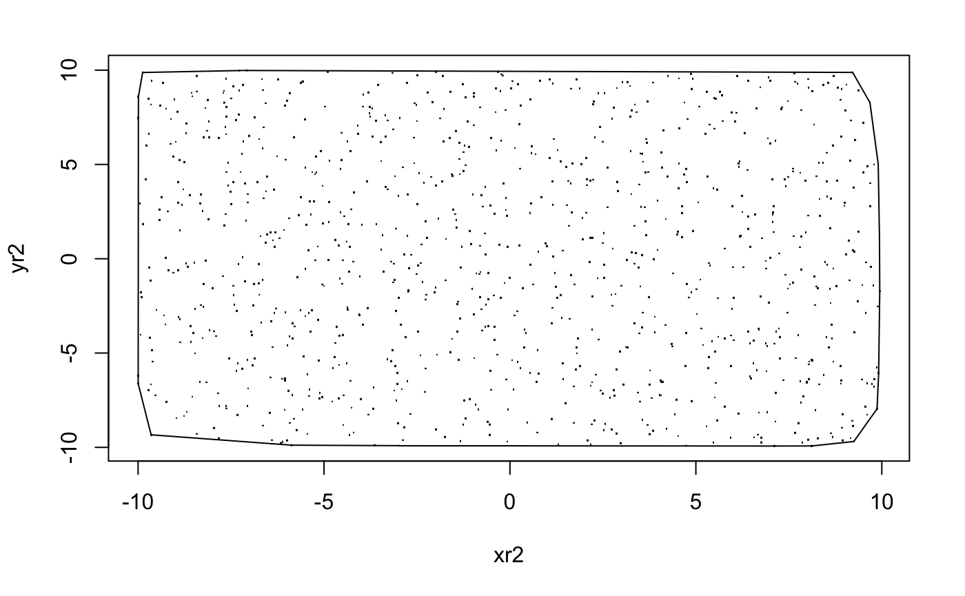
plot(xr2,yr2,pch=".")
polygon(xr2[inx],yr2[inx])area_mc_method_v4(xr2[inx],yr2[inx],plotpoly = FALSE,typepoly = FALSE)## [1] 390.754Also it's worth to notice that, if we generate the points over a rectangle uniformly, then the area of convex hull will approximately the same as the area of the rectangle. As we uniformly generate those points, there must be points around four corners, so the convex hull just looks like the rectangle itself. So we can say, if we generate $n$ points, as $n$ tends to infinity, the convex hull will tends to the region used to generate the points.
Apart from finding the convex hull, we can use the type of polygon function to test a large set of points. For example, if the first 5 points form a convex polygon, but the six points will make it self-intersecting or becomes concave, then we skip the point and move on to the next one. Code would look like this:
k2 <- 1000 # Number of points
bad_point_x <- c()
bad_point_y <- c()
xr1 <- runif(k2,-10,10)
yr1 <- runif(k2,-10,10)
for (i in 3:k2) {
  if (length(bad_point_x) == 0) {
    if (type_of_polygon(xr1[1:i], yr1[1:i]) != "Convex") {
      bad_point_x <- c(bad_point_x, i)
      bad_point_y <- c(bad_point_y, i)
    }
  } else {
    if (type_of_polygon(xr1[1:i][-bad_point_x], yr1[1:i][-bad_point_y]) != "Convex") {
      bad_point_x <- c(bad_point_x, i)
      bad_point_y <- c(bad_point_y, i)
    }
  }
  if (i == k2) {
    plot(xr1,yr1, pch = ".")
    polygon(xr1[1:i][-bad_point_x],yr1[1:i][-bad_point_y])
  }
}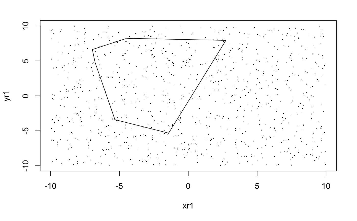
However, the limitation is very obvious. This method normally fails with a lot of "bad points" at the end.
Also, we can reorder the points: Instead of the given order, the furthest point from the centre of the set of points will be the first one, and the nearest one will be the last one. Then the method above will likely return a larger polygon.
k2 <- 1000 # Number of points
bad_point_x <- c()
bad_point_y <- c()
xr1 <- runif(k2,-10,10)
yr1 <- runif(k2,-10,10)
mean_xr1 <- mean(xr1)
mean_yr1 <- mean(yr1)
ordered_xr1 <- c()
ordered_yr1 <- c()
for (i in 1:k2) {
  ordered_xr1[i] <- xr1[sort((xr1 - mean_yr1)^2 + (yr1 - mean_yr1)^2, decreasing = TRUE, index.return = TRUE)$ix[i]]
  ordered_yr1[i] <- yr1[sort((xr1 - mean_yr1)^2 + (yr1 - mean_yr1)^2, decreasing = TRUE, index.return = TRUE)$ix[i]]
}
for (i in 3:k2) {
  if (length(bad_point_x) == 0) {
    if (type_of_polygon(ordered_xr1[1:i], ordered_yr1[1:i]) != "Convex") {
      bad_point_x <- c(bad_point_x, i)
      bad_point_y <- c(bad_point_y, i)
    }
  } else {
    if (type_of_polygon(ordered_xr1[1:i][-bad_point_x], ordered_yr1[1:i][-bad_point_y]) != "Convex") {
      bad_point_x <- c(bad_point_x, i)
      bad_point_y <- c(bad_point_y, i)
    }
  }
  if (i == k2) {
    plot(ordered_xr1,ordered_yr1,pch=".")
    polygon(ordered_xr1[1:i][-bad_point_x],ordered_yr1[1:i][-bad_point_y])
  }
}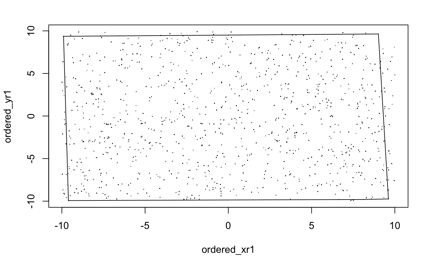
But like the first one, this method normally fails with a lot of "bad points" at the end. Figure 8.3 is just an ideal example from the code above. It doesn't mean we can't do something, like set a while loop inside, detect the area. If the area is less than, like 90% of the rectangle, then repeat until the area is larger than that.
It is also possible to use the type of polygon function to generate a random simple polygon. Just put it into a while loop, and keep generating points inside a region. If the point generated form a convex/concave polygon in the given order, then stop the while, else repeat the process.
generate_poly <- function(n, convex = TRUE) { # Must faster if convex is TRUE
  simple <- FALSE
  while (!simple) {
    x <- runif(n,-2,2) # If convex n < 9, if !convex n < 7
    y <- runif(n,-2,2)
    if (!convex) type <- type_of_polygon_v2(x,y) else if (convex) type <- type_of_polygon(x,y)
    if (!convex) {
      if (type == "Convex" || type == "Concave") {
        plot(x,y,asp = 1,pch = "")
        polygon(x,y)
        simple <- TRUE
      }
    } else if (convex) {
      if (type == "Convex") {
        plot(x,y,asp = 1,pch = "")
        polygon(x,y)
        simple <- TRUE
      }
    }
  }
  return(list(x = x, y = y))
}
Like the function above, it generates a $n$-side polygon randomly. But when $n$ gets larger, it will be extremely slow, so $n \leq 8$ is recommended.
generate_poly(8) # n = 6 with convex = FALSE is terrible already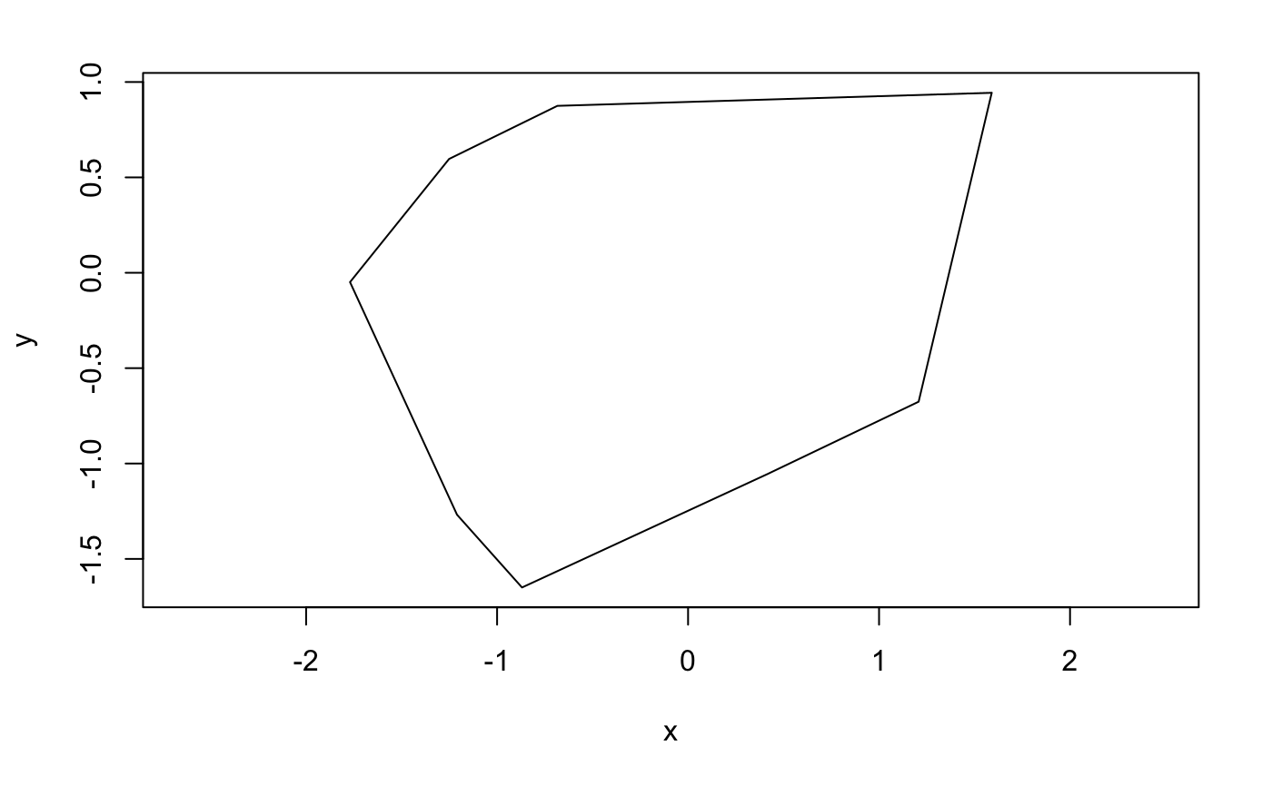
## $x
## [1]  1.5902308 -0.6844604 -1.2514097 -1.7701839 -1.2096977 -0.8694716  0.4245622  1.2072511
##
## $y
## [1]  0.94380260  0.87501177  0.59655934 -0.04909636 -1.26849916 -1.64980162 -1.05089891 -0.67585441
We can also generate a random polygon by setting a centre point first, and then span the angle and distance from the point randomly, also limit the sum of angle to $2\pi$. This method is much faster and it works very well, we can also use it to generate lattice polygon and calculate the area by Pick's theorem.
generate_poly_v2 <- function(n, area=FALSE, int = FALSE) { # If int, pls not make n too large
  r <- c()
  angle <- c()
  x <- c()
  y <- c()
  for (i in 1:n) {
    r[i] <- runif(1,0.5,1.5)
    angle[i] <- runif(1,0.9*2*pi/n,1.1*2*pi/n)
  }
  cumangle <- cumsum(angle)
  if (int) {
    for (i in 1:n) {
      x[i] <- round(4*r[i]*cos(cumangle[i]))
      y[i] <- round(4*r[i]*sin(cumangle[i]))
    }
    grad <- gradient(x,y)
    inx <- c(n+1)
    nan_grad <- FALSE
    for (i in 1:n) {
      if (is.nan(grad[i])) {
        inx <- c(inx,i)
        nan_grad <- TRUE
      }
    }
    x <- x[-inx];y <- y[-inx]
    x2 <- start_from_minx_v2(x,y)$x
    y2 <- start_from_minx_v2(x,y)$y
  } else for (i in 1:n) {
    x[i] <- r[i]*cos(cumangle[i])
    y[i] <- r[i]*sin(cumangle[i])
  }
  if(area) {
    if (int) return(picks_theorem(x2,y2)) else return(area_mc_method_v4(x,y))
  } else plot(x,y,pch="");polygon(x,y)
}
Example 8.1 Generate a random simple lattice polygon and find the area by Pick's Theorem.
generate_poly_v2(20,area=TRUE,int=TRUE) # Too large n might cause self-intersecting polygon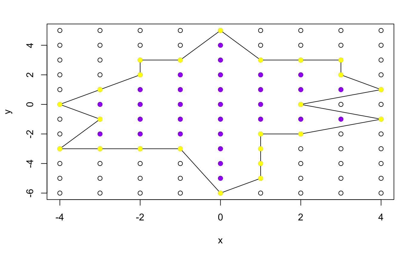
## [1] 41Or else, we can use Monte Carlo method to find the area of the random polygon.
Example 8.2 Generate a random simple polygon and find the area by Monte Carlo method.
generate_poly_v2(20,area = TRUE)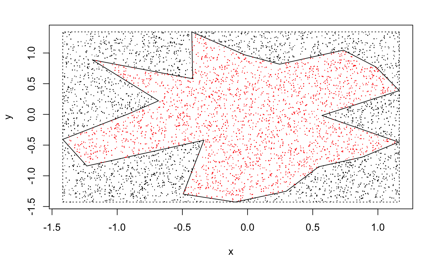
## [1] 3.732384© Group 18