Now we talk about some algorithms that widely known in computer science and mathematics. To determine a point is inside or outside the polygon, there are two popular algorithms: Ray-casting algorithm [7] and Winding number algorithm.[20]
If there is a ray starting from a point $O$, the number of times that the point $O$ passing the edges of polygon can be used to decide whether the point $O$ is inside or outside. Imagime a convex polygon, and if a point is inside there, then whatever direction the ray is pointing, it will only pass the edge once. If not, it will pass none or twice.
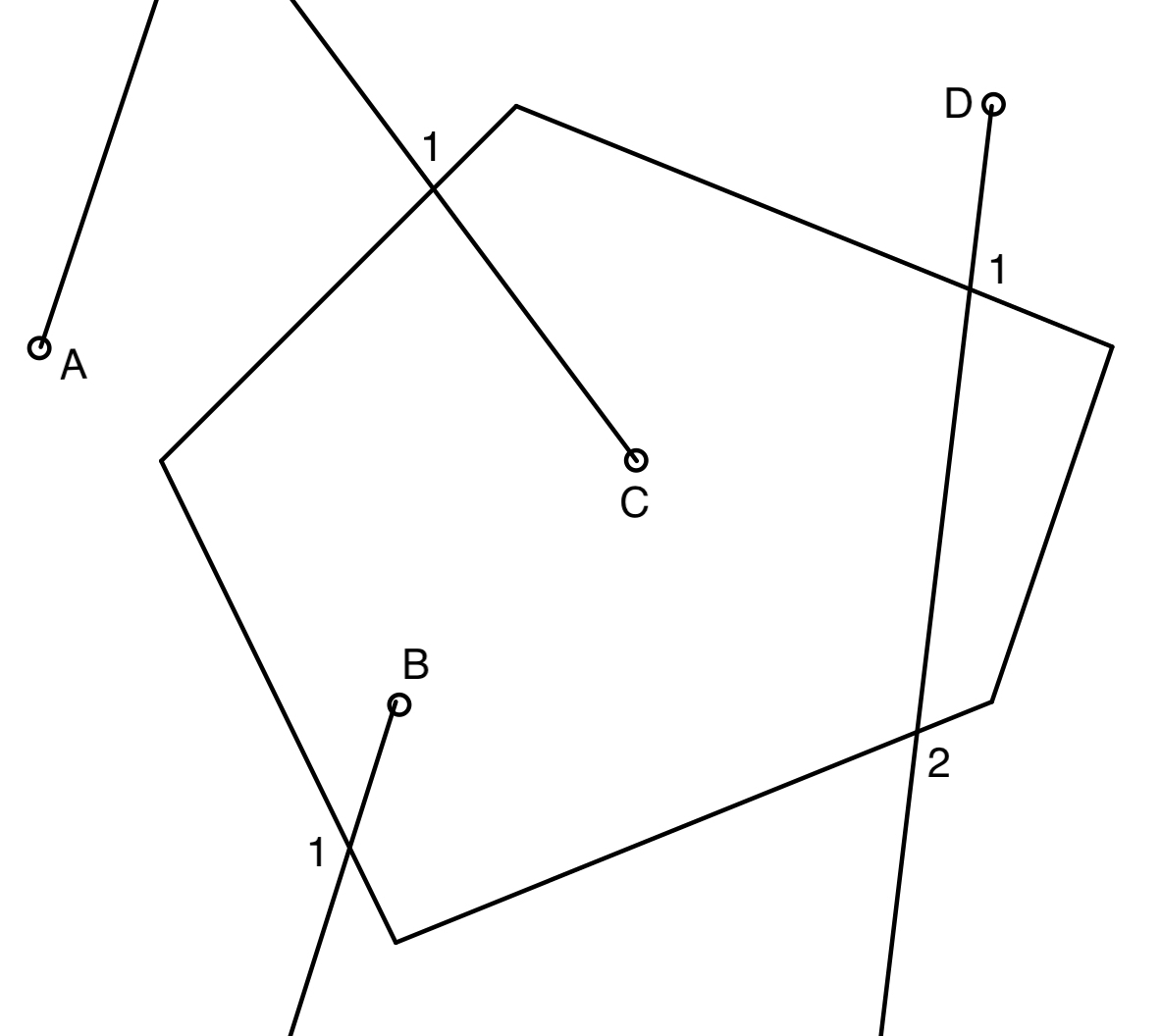
In Figure 4.1, point $A$ and $D$ are outside the polygon, point $B$ and $C$ are inside the polygon. It is obvious that the rays from point $B$ and $C$ only pass the edge of the polygon once, but the ray from point $D$ passes twice. Also, the ray from point $A$ doesn't pass the polygon.
For a point in concave polygon, there exists another situation: The ray passes one edge and through the polygon again.
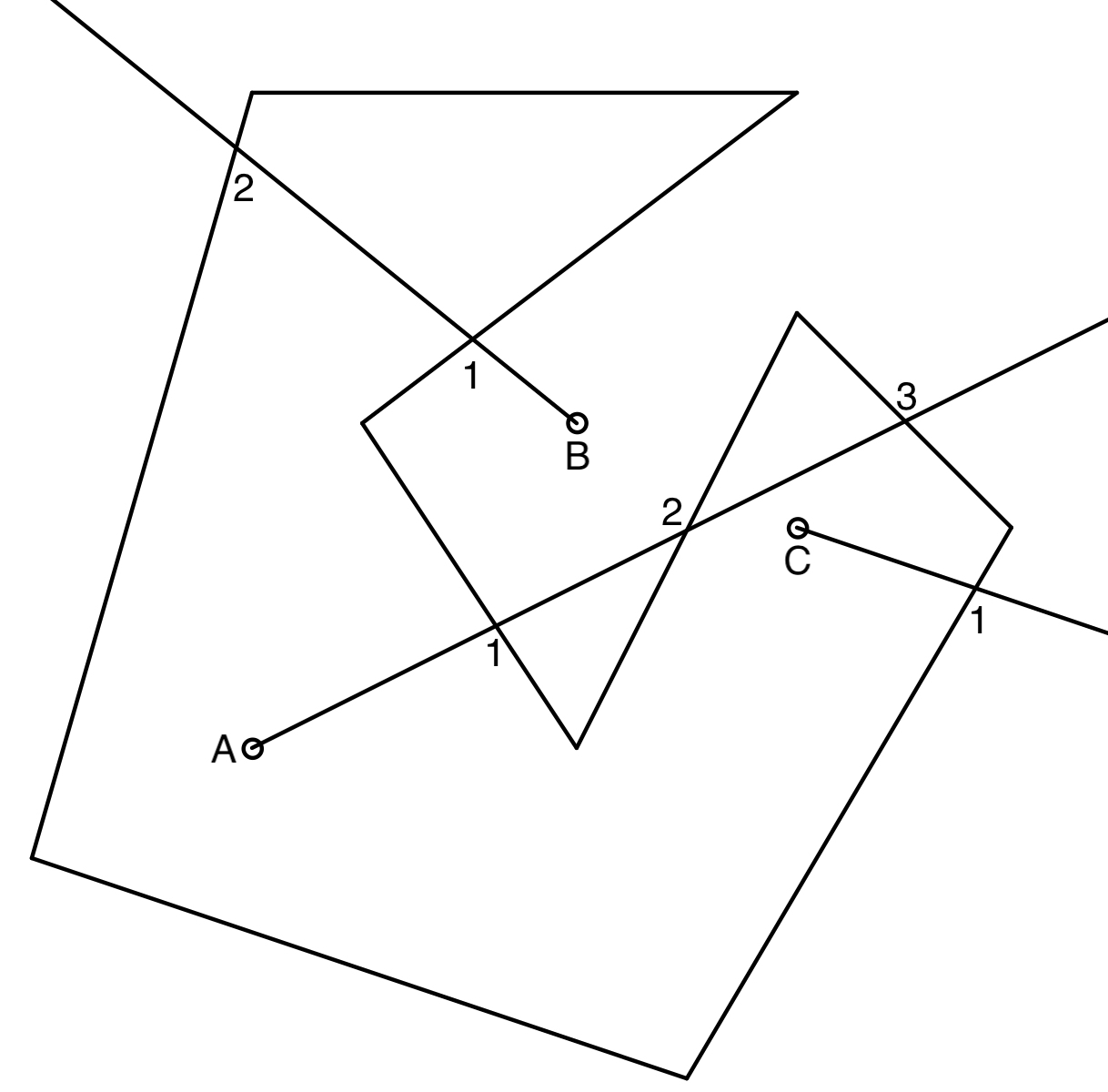
In Figure 4.2, point $A$ and $C$ are inside the polygon, point $B$ is outside the polygon. We can observe that the ray from point $A$ passes the edges of the polygon three times. Because it is inside the polygon, then the ray should leave the polygon first, and might enter and leave the polygon.
For a point in self-intersecting polygon, the ray might just pass the intersection point of the polygon, which seems like the wrong result will occur. But it is possible to consider that in the code and get the correct result. Actually, that would be the same as passing the vertex but not enter the convex or concave polygon.
One possible solution is, if the ray passes the intersection point, then count it twice. However, instead of casting one ray, it is better to cast more rays in different directions, and check the parity of each ray.
In the previous session, there is a function called line_equ to find the corresponding $y$-coordinate of a point on a line by given the $x$-coordinate. Then we can rewrite that function from $y=f(x)$ to $x=g(y)$ by changing the order:
line_equy <- function(x,y) {
  fy <- c()
  grad <- gradient(x,y)
  n <- length(x)
  f <- function(i) {
    g <- grad[i] # We can avoid to use the case when gradient is Inf or -Inf
    xm <- x[i]
    ym <- y[i]
    function(y) (y - ym)/g + xm
  }
  for (i in 1:n) { #  In case input the same vertex twice or more
    if (is.nan(grad[i])) {
      return(cat("Input values are not vaild, repeat points detected."))
    }
    fy <- c(fy,f(i))
  }
  return(fy)
}
linen_equy <- function(x,y,n) {
if(n == 0) {
return(line_equy(x,y)[[length(y)]])
} else if (n > length(y)) {
n1 <- n %% length(y)
return(line_equy(x,y)[[n1]])
} else {
return(line_equy(x,y)[[n]])
}
}With this function, we can easily find the correspoinging $x$-coordinate if the $y$-coordinate is given. Which will be very useful if we cast a ray from a point to the right. The line equation of the ray from point $(x_0,y_0)$ horizontally to the $x$-axis is $y=y_0$, so only the $y$-coordinate is known.
Now convert the algorithm into a function:
ray_pass <- function(x,y,x0,y0) {
  pass_x <- c() # Rightward ray, passing point x-coordinate
  pass_x2 <- c() # Leftward ray
  pass_pi <- c() # π/4 rad ray
  n <- length(x) # Number of vertices
  x2 <- x;x2[n+1] <- x2[1]
  y2 <- y;y2[n+1] <- y2[1]
  grad <- gradient(x,y) # Gradient of each edge in the polygon
  for (i in 1:n) {
    if (grad[i] == 0) next else if (abs(grad[i]) != Inf) {
      if (y0 <= max(y2[i],y2[i+1]) && y0 >= min(y2[i],y2[i+1])) {
        if (linen_equy(x,y,i)(y0) >= x0) pass_x <- c(pass_x,linen_equy(x,y,i)(y0))
        else pass_x2 <- c(pass_x2,linen_equy(x,y,i)(y0))
      }
    } else {
      if (y0 <= max(y2[i],y2[i+1]) && y0 >= min(y2[i],y2[i+1])) {
        if (x0 <= x2[i]) pass_x <- c(pass_x,x2[i])
        if (x0 >= x2[i]) pass_x2 <- c(pass_x2,x2[i])
      }
    }
  }
  if ((length(pass_x) %% 2) == (length(pass_x2) %% 2)) return(length(pass_x))
  if ((length(pass_x) %% 2) != (length(pass_x2) %% 2)) {
    for (i in 1:n) {
      if (grad[i] == 0) next else if (abs(grad[i]) != Inf) {
        xi <- seq(min(x2[i],x2[i+1]),max(x2[i],x2[i+1]),length.out=(floor(abs(x2[i]-x2[i+1]))*1000+1))
        for (j in xi) {
          if (abs(linen_equ(x,y,i)(j) - (j - x0 + y0)) < 0.001) {
            if (x0 <= j) pass_pi <- c(pass_pi,j)
            break
          }
        }
      } else {
          if ((x2[i] - x0 + y0) <= max(y2[i],y2[i+1]) && (x2[i] - x0 + y0) >= min(y2[i],y2[i+1])) {
          if (x0 <= x2[i]) pass_pi <- c(pass_pi,x2[i])
        }
      }
    }
    return(length(pass_pi))
  }
}
This function is another looks long but simple function, it just like actually casting a ray from a point $(x_0,y_0)$ toward the right, and counting the edges it passes. It works for all kind of polygon, and try to minimise the error. It will cast two rays, one leftward and one rightward. If the parity of the number of intersections are different, then it will cast another ray $\pi/4$ rad upward and take that as the final result. There's still possible that a point inside passes the polygon even number times after all, but the possibility is insignificant.
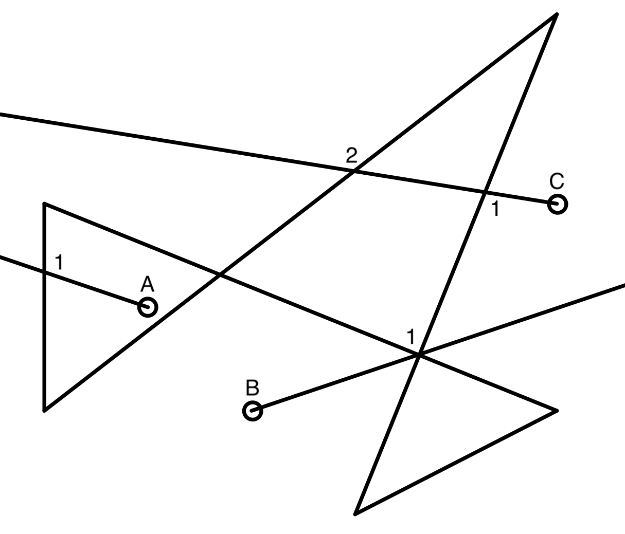
We can clearly see that, in Figure 4.4, the rays cast from point $A$ rightward passing a vertex and an edge, same as the ray leftward. The number of passing the edge should be both $3$ in this case, which means point $A$ is inside the polygon. However, the downward ray from point $C$ has the passing number 2, and the upward ray has the passing number 6, which means point $C$ is outside the polygon. But that's wrong, as point $C$ is indeed inside.
The reason behind this problem is, the rays from point $A$ is "passing" the vertex and leaving the polygon, whereas the downward ray from point $C$ is leaving the polygon via the vertex, so we should only count it once. Similar to point $B$, as entering the polygon via a vertex should not be counted twice.
To reduce this happens, in the function it will cast two to three rays, which will greatly avoid the "passing vertex" cases happen. For example, if we test the function with point $B$ in Figure 4.4, then it will first calculate the passing number of the rays toward left and right at the same time, and the counting number are $3$ and $4$ respectively. Since they are not the same, it will calculate the passing number of the ray $\pi/4$ rad upward, which is $2$. Then the function will take it as the final result.
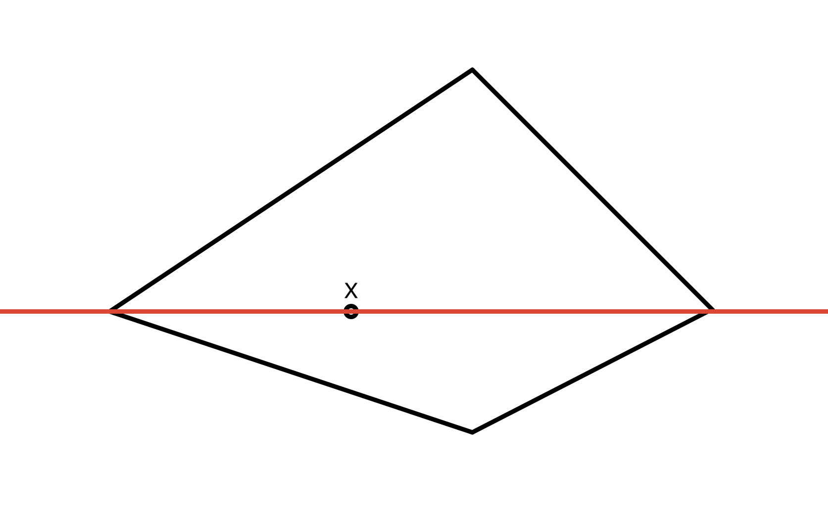
But in Figure 4.5, point $X$ would be outside the polygon if test it with the function. That's because the left and right ray will both meet a vertex when leaving the polygon, and have counted it twice.
Although it is still possible to meet the wrong result, it is not supposed to affect the estimate area too much, as explain before the insignificant of the possibility. More importantly, we are going to generate a number of points randomly and uniformly, which makes it harder to have a ray actually passing any vertex.
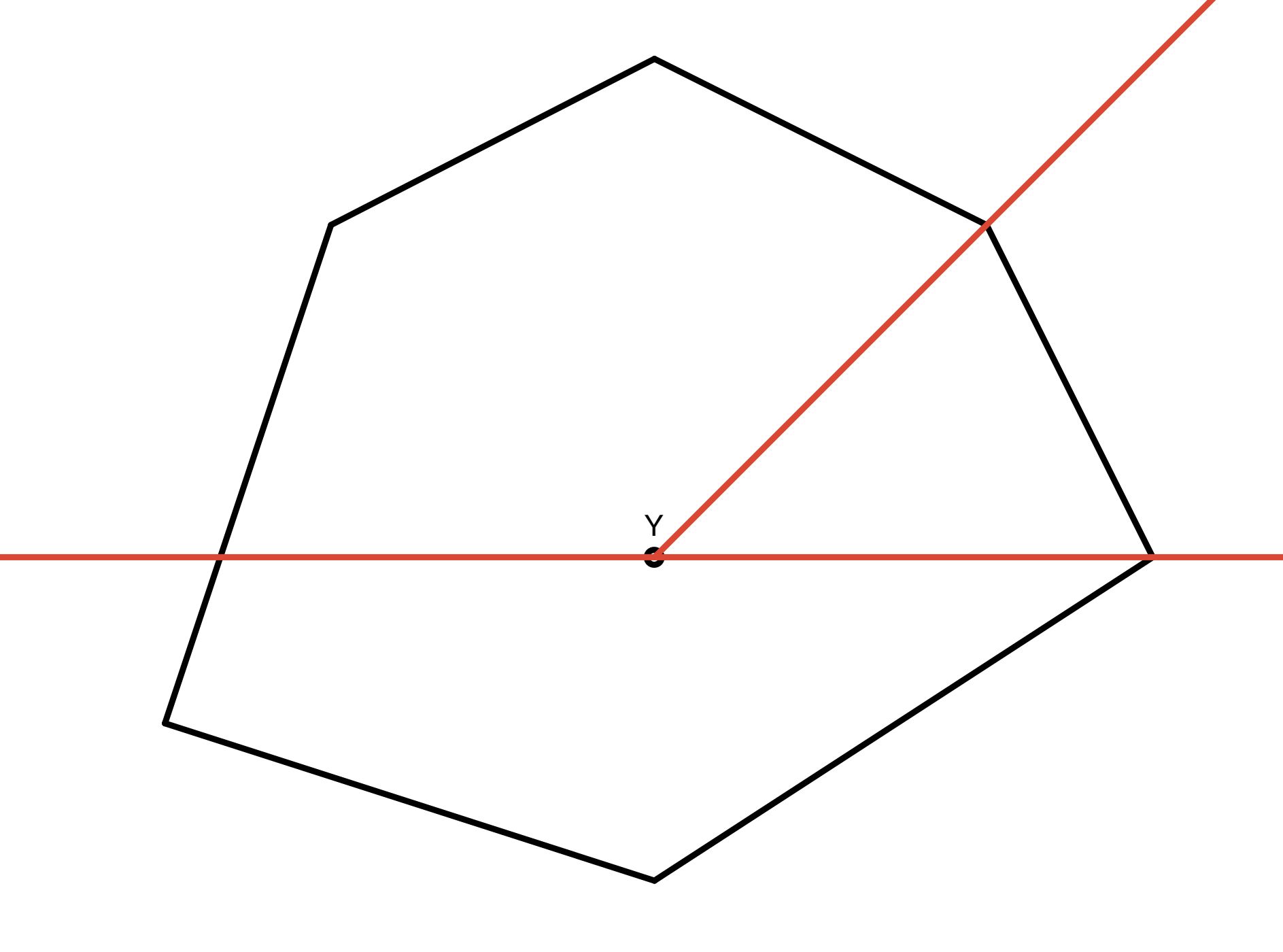
Figure 4.6 shows another possible bug, but this is much harder to be happened.
The winding number of a closed planar curve $C$ for a point $\mathbf{x}$ is the number of times that the curve $C$ winds round $\mathbf{x}$ in anticlockwise rotation. Therefore the winding number is signed, positive means anticlockwise winding, negative means clockwise winding.
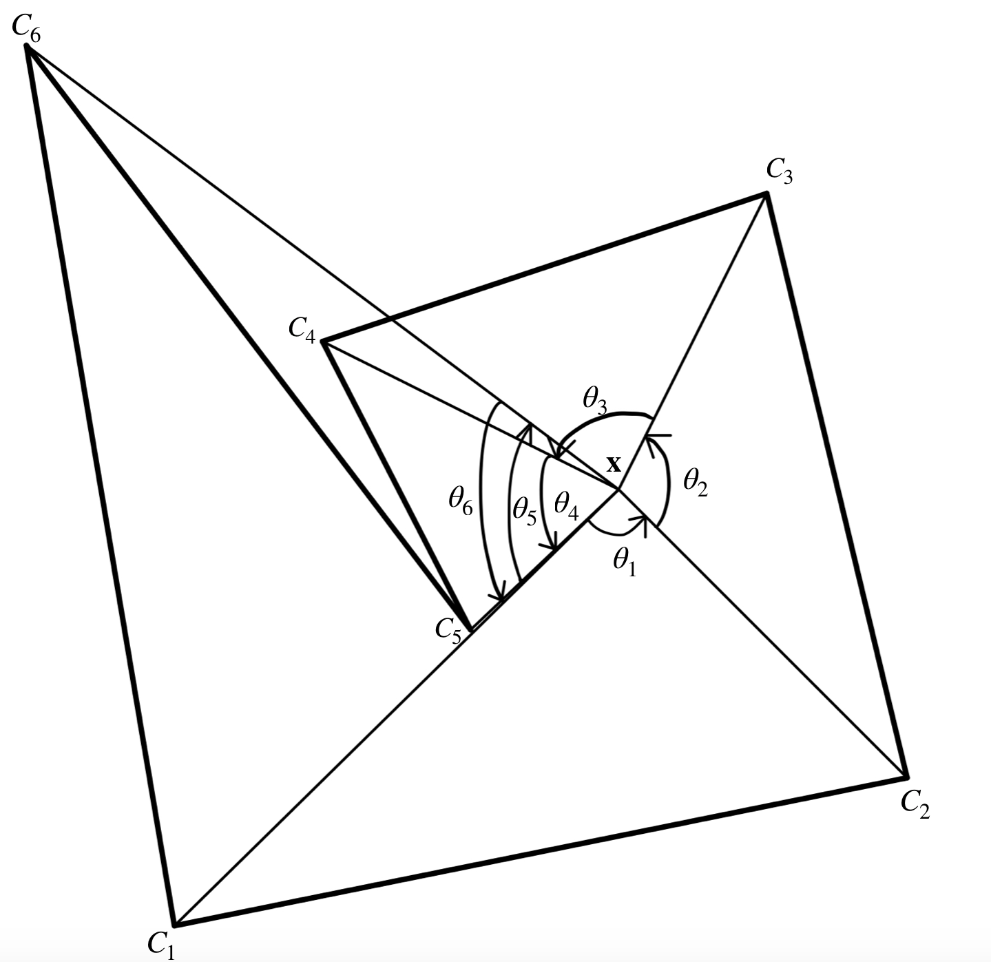
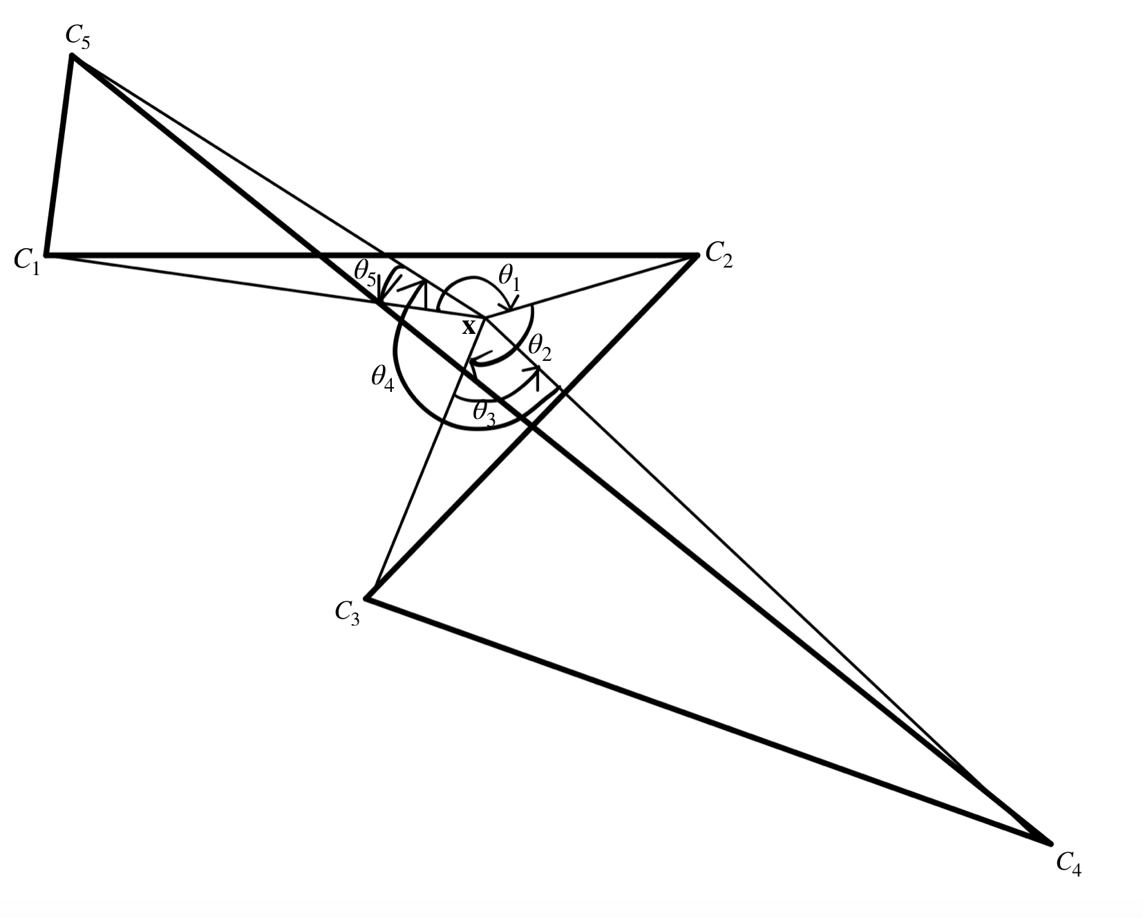
We can calculate the winding number by measuring the angle winded. Remember the angle also have its direction: Anticlockwise rotation is positive, clockwise is negative. If we want to find the winding number of a point relate to a polygon, the best technique is to set the first vertex $\mathbf{C_1}$ as the starting point, and then find the angle between the point and vertices. For example:
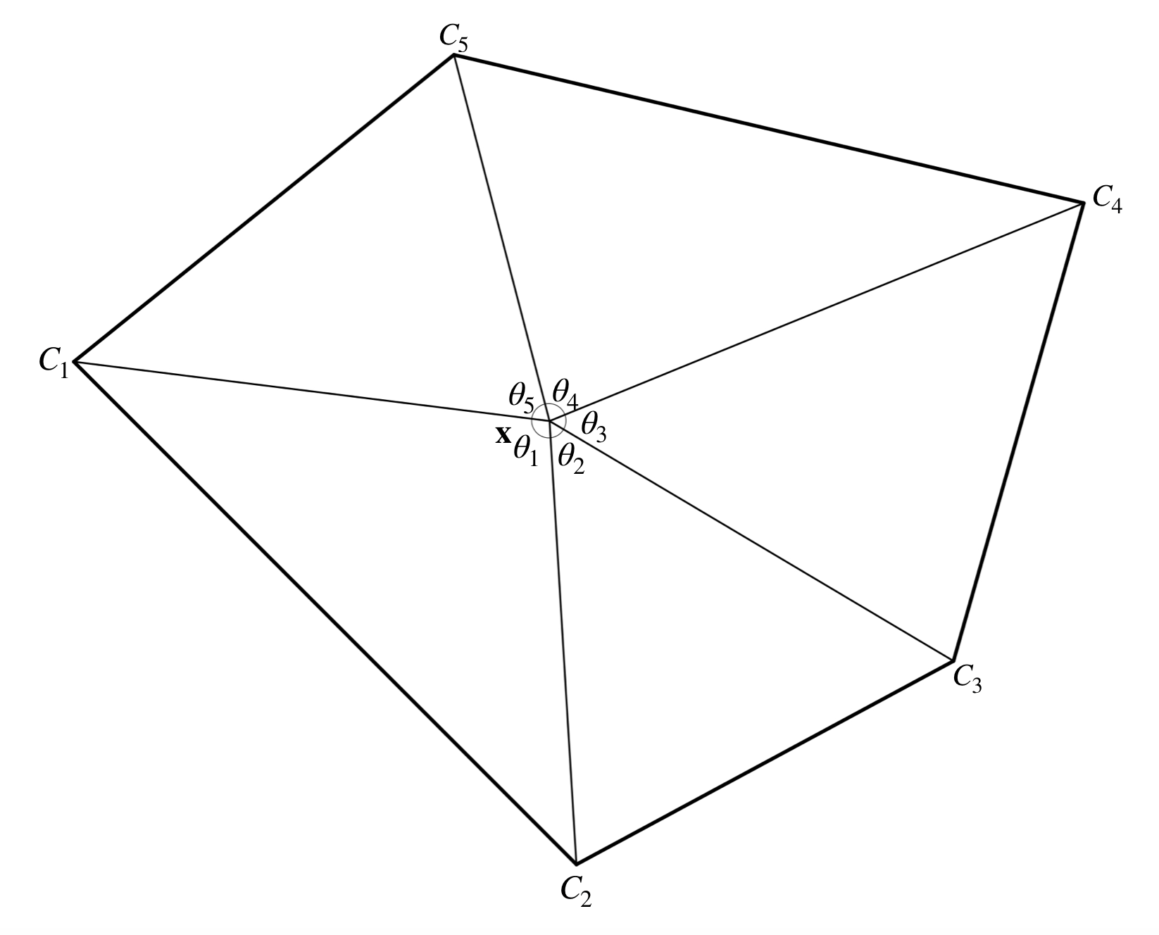
As the rotation starts from $C_1$ in anticlockwise, the total angle rotated is $\sum_{i=1}^{5}\theta_i = 2\pi$ and hence the winding number is $1$.
Since the angle of a complete rotation is $2\pi$ in anticlockwise, the winding number can be calculated as the angle rotated divided by $2\pi$. Let's see another example where the point is outside the polygon:
If a point is outside the polygon, as Figure 4.8, the winding number will be $0$ as the angle rotated is $0$.
Similarly, point inside the concave polygon has the winding number $1$, as the sum of the anticlockwise angles and clockwise angles is $2\pi$.
But the key problem is, how to convert this algorithm into a function in R.
First of all, if the point is lying at the border of the polygon, then we still consider the point is inside the polygon. Which means, the expected winding number of such point is non-zero. In Figure 4.7, we can simply add the angle of the rotation to get the total rotation angle, but in Figure 4.8 it is not possible to do that, because the angle we calculate by scalar product is always positive.
The recommended way we can use to find the angle between two vectors is the scalar product, but it only return the positive value between $0$ and $\pi$, which is another limitation. There are still some solutions, like compare the cumulative sum of first $i$ angles and the angle between the line $C_1 \mathbf{x}$ and $C_{i+1} \mathbf{x}$. But again, if the sum of the angle is lager than $\pi$, whcih will be another problem.
The angle we want to find is relative to the given point $\mathbf{x}$, and that point is randomly generate later when applying the Monte Carlo method. Then we can write a function to find out the angle between vertices and the ray start from the given point rightward, and use that to figure out is the rotation angle is positive or negative, i.e. anticlockwise or clockwise rotation.
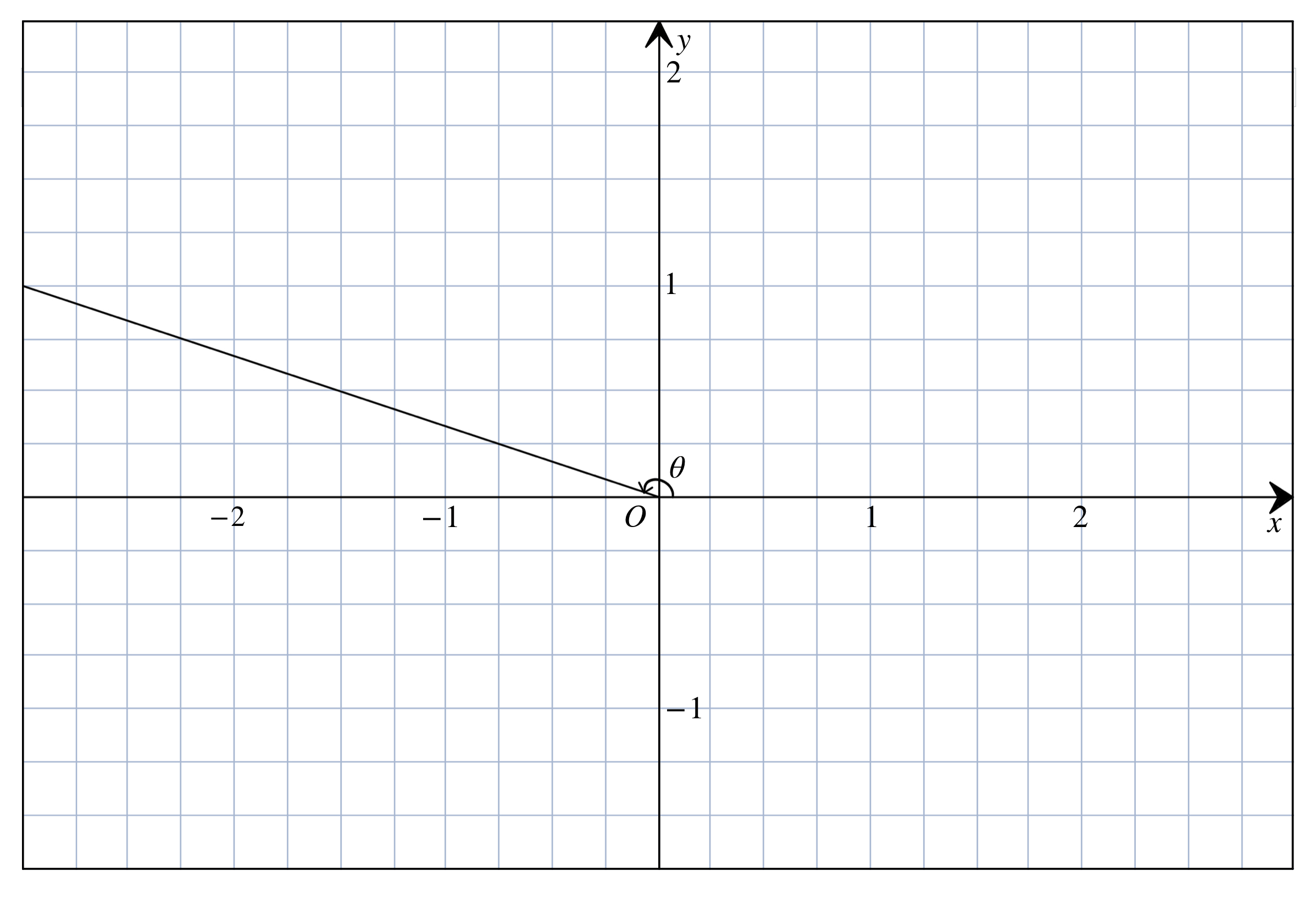
However, the built-in function atan in R can only return the angle between $-\frac{\pi}{2}$ and $\frac{\pi}{2}$, so if we want to calculate the obtuse angle in Figure 4.10, we will have to add $\pi$ into the result.
atan(1/-3) # Change in y over change in x## [1] -0.3217506atan(1/-3) + pi## [1] 2.819842Similarly, for the reflex angle between $\frac{3}{2}\pi$ and $0$, it will return the negative value, which we need to add $2\pi$ into it.
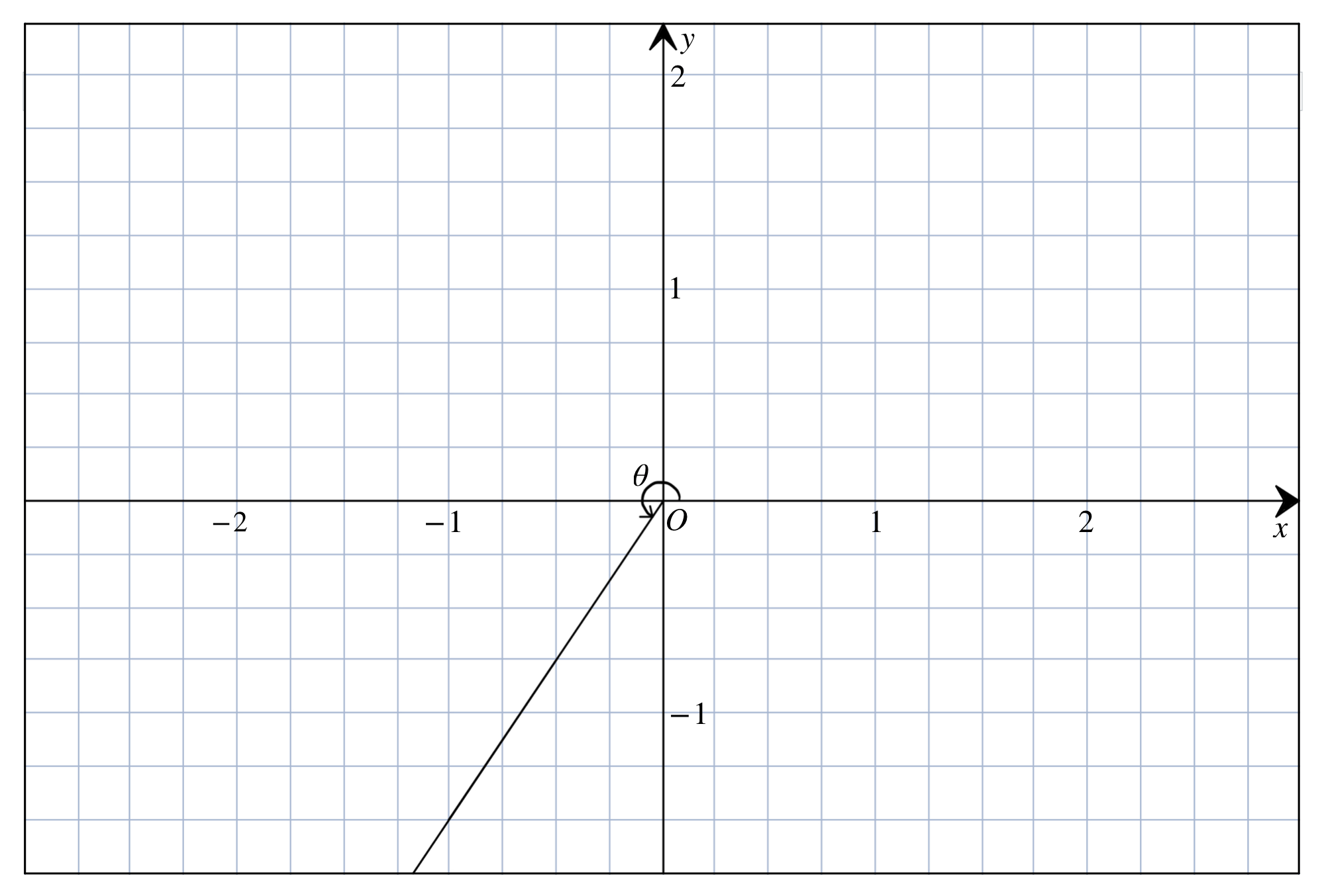
For the reflex angle between $\pi$ and $\frac{3}{2}\pi$, like the one in Figure 4.11, again we need to add $\pi$ into the result.
atan(-2/-3) # Change in y over change in x## [1] 0.5880026atan(-2/-3) + pi## [1] 3.729595Finally, if the point lies on the axes, then return the specific angle. What about if the point lies on the origin? Well in the winding number algorithm, we define that if the point is lying at the border of the polygon, then we still consider the point is inside the polygon before. Which is, we don't need to calculate the angle if the point is at the vertex.
Now summarise into a function:
angle <- function(x0,y0,rx,ry) {
  if (y0 == ry) {
    if (x0 >= rx) return(0) else return(pi)
  } else if (y0 > ry) {
    if (x0 == rx) return(pi/2)
    else if (x0 > rx) return(atan((y0 - ry)/(x0 - rx)))
    else return(pi + atan((y0 - ry)/(x0 - rx)))
  } else {
    if (x0 > rx) return(2*pi + atan((y0 - ry)/(x0 - rx)))
    else if (x0 < rx) return(pi + atan((y0 - ry)/(x0 - rx)))
    else return(3*pi/2)
  }
}
In angle function, there are 4 variables: x0,y0 means the coordinate of vertex, and rx,ry means the coordinate of randomly generated point. It will return the angle between the vertex and the rightward ray start from a given point.
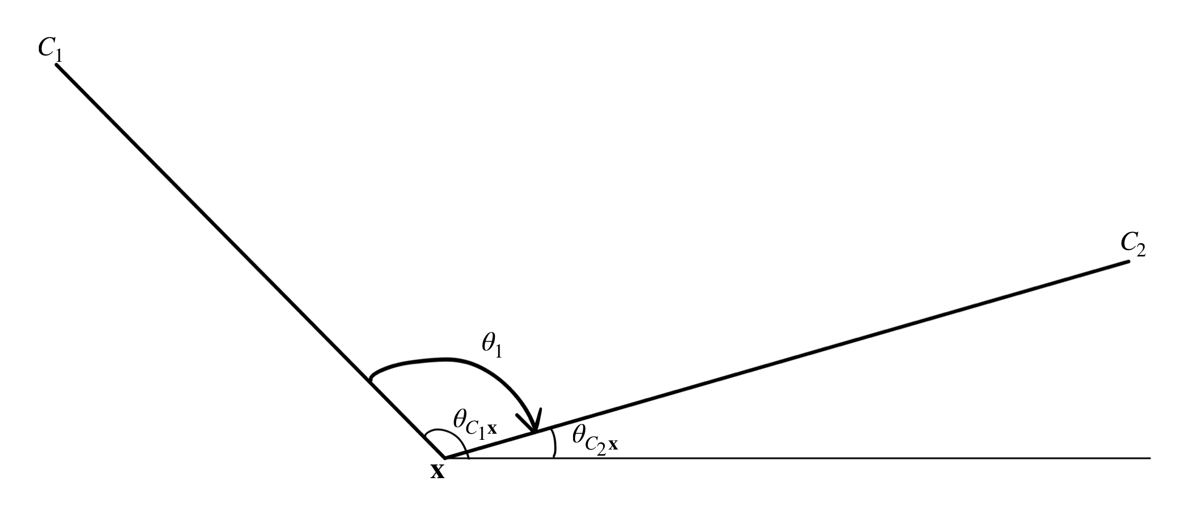
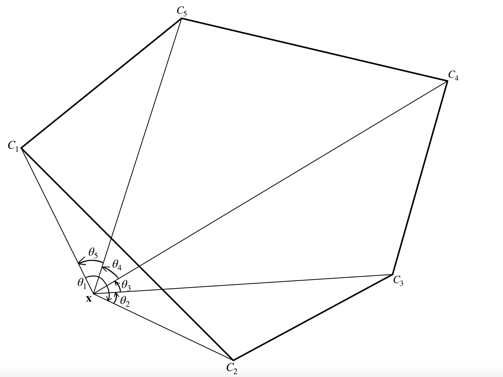
In Figure 4.12, angle between $C_1$ and the line from $\mathbf{x}$ in positive $x$-direction is larger than angle between $C_2$ and the line from $\mathbf{x}$ in positive $x$-direction, which means it is clockwise rotation. But this is just a simple case, because if the point $C_2$ is under the line, then angle $\theta_{C_2\mathbf{x}}$ will be larger than angle $\theta_{C_1\mathbf{x}}$, but still in clockwise rotation.
Just like the winding in Figure 4.13, from $C_2$ to $C_3$ the rotation pass the line from $\mathbf{x}$ in positive $x$-direction, but notice that the difference between $\theta_{C_3\mathbf{x}}$ and $\theta_{C_2\mathbf{x}}$, i.e. $\theta_{C_3\mathbf{x}} - \theta_{C_2\mathbf{x}}$ is larger than $\pi$, so it is clockwise.
But what about the rotation from $C_3$ to $C_2$? It is anticlockwise, and $\theta_{C_2\mathbf{x}}-\theta_{C_3\mathbf{x}}$ is smaller than $-\pi$.
Clearly it is possible to deduce the clockwise or anticlockwise rotation between two vertices about a point, and below is the summary for the rotation from $C_1$ to $C_2$:
if (c2x - c1x >= pi || (c2x - c1x > -pi && c2x - c1x < 0)) anti <- FALSE
else if ((c2x - c1x < pi && c2x - c1x >= 0) || c2x - c1x <= -pi) anti <- TRUE
where c1x,c2x means the same thing as $\theta_{C_1\mathbf{x}}$ and $\theta_{C_2\mathbf{x}}$.
Once we know the direction of the rotation, we can simply plus or minus the angle during the winding around the point $\mathbf{x}$, depends on the clockwise or anticlockwise rotation. Below is the function to find out the windind number for a point $(x_0,y_0)$ inside the polygon.
winding_number <- function(x,y,x0,y0) {
  cumang <- 0
  direction <- list()
  anglex <- c()
  n <- length(x)
  for (i in 1:n) {
    direction <- c(direction,list((c(x0,y0) - c(x[i],y[i]))))
    anglex <- c(anglex, angle(x[i],y[i],x0,y0))
  }
  direction[n+1] <- direction[1]
  anglex[n+1] <- anglex[1]
  anti <- TRUE
  for (i in 1:n) {
    if (norm(direction[[i]])*norm(direction[[i+1]]) == 0) return(1)
    if (anglex[i+1] - anglex[i] > pi || (anglex[i+1] - anglex[i] > -pi && anglex[i+1] - anglex[i] < 0)) anti <- FALSE
    else if ((anglex[i+1] - anglex[i] < pi && anglex[i+1] - anglex[i] >= 0) || anglex[i+1] - anglex[i] <= -pi) anti <- TRUE
    dotproduct <- as.numeric(direction[[i]] %*% direction[[i+1]])
    nomproduct <- norm(direction[[i]])*norm(direction[[i+1]])
    angle <- acos(round(dotproduct/nomproduct,8))
    if (anti) cumang <- cumang + angle else cumang <- cumang - angle
  }
  wind <- round(cumang/(2*pi))
  return(wind)
}
If the point $(x_0,y_0)$ is at the vertex, then the direction vector between them is $\mathbf{0}$, also the norm is $0$. So if the norm of the direction vector is $0$, then the function will return the winding number $1$, in order to avoid the NaN appears. If not, then the function will use the technique of dot product to calculate the angle. If it is clockwise rotation, the function will subtract the angle from the cumulative sum of the angle, else the function will add the angle into the cumulative sum of the angle.
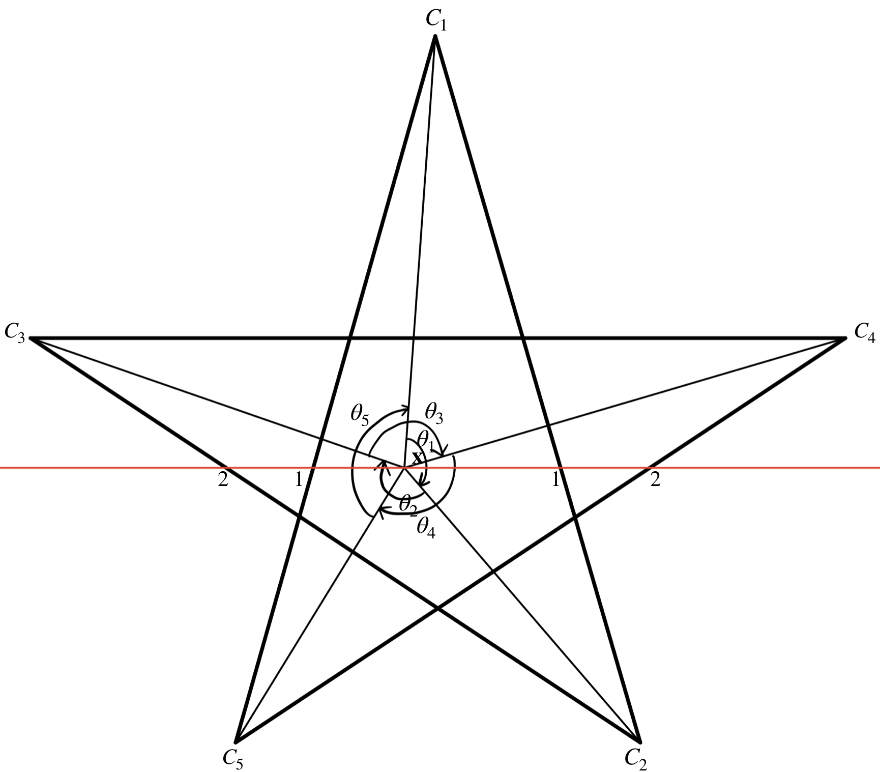
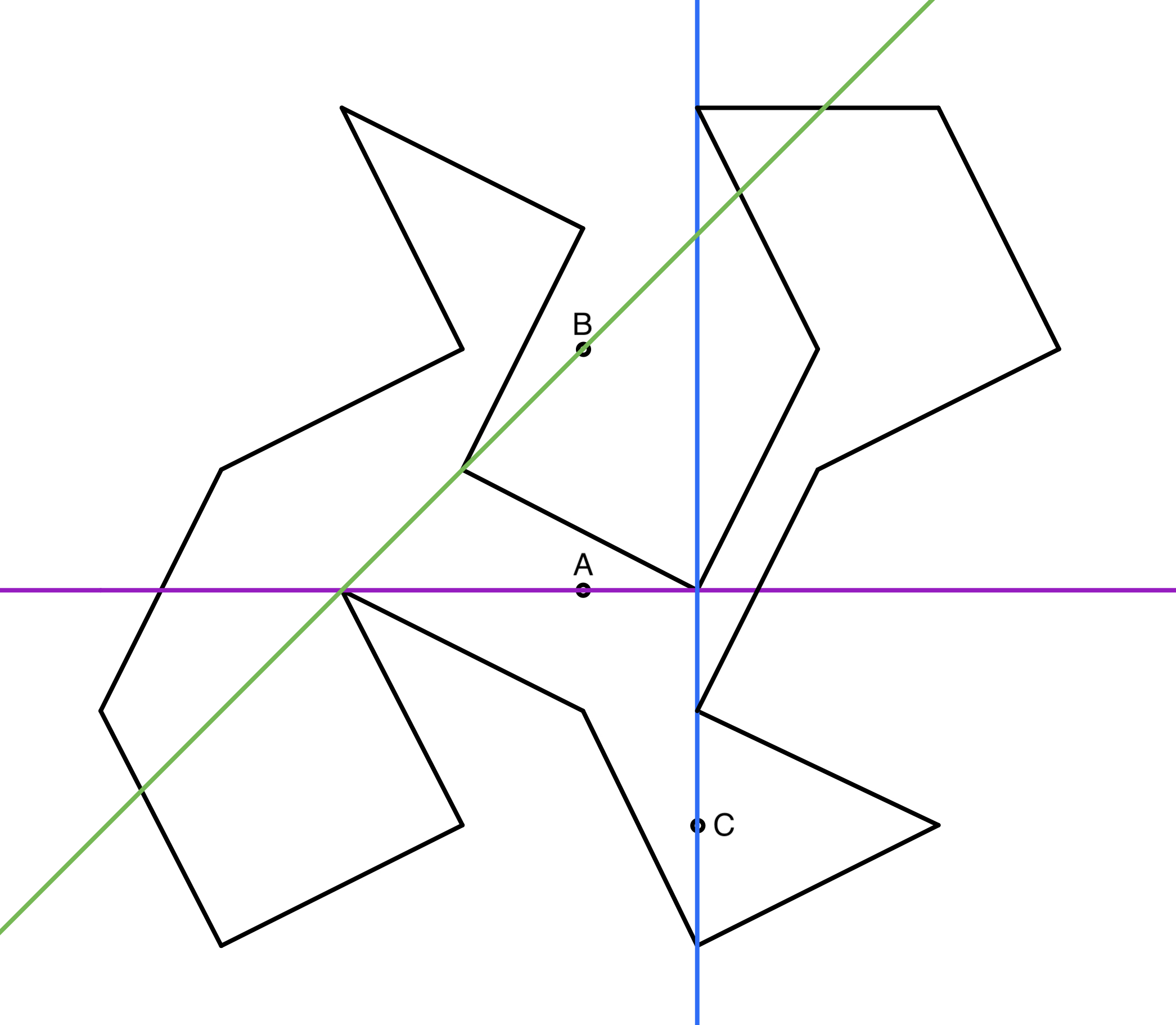
But one possible problem is, if the polygon is pentagram, then what about the central pentagon region? If a point is inside there, should we consider that is inside the polygon or not? Like the point in Figure 4.14, It looks like it is inside the polygon, but if we cast a ray, it will "enter" and "exit" the polygon. However, if we count the winding number, the winding number will be $-2$, which is inside the polygon.
However, that's not a big problem. We can consider both as two separate cases, and it actually depends on the requirement.
xe0 <- c(4,6,0,8,2)
ye0 <- c(3,-4,0,0,-4)
area_mc_method_v3(xe0,ye0,method = "wind")
## [1] "Self-intersecting Polygon"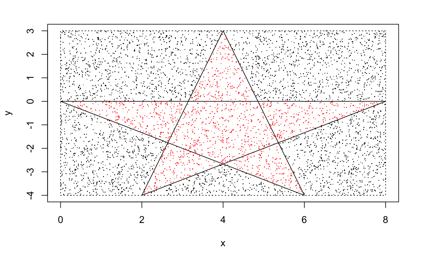
## [1] 16.7328xe0 <- c(4,6,0,8,2)
ye0 <- c(3,-4,0,0,-4)
area_mc_method_v3(xe0,ye0,method = "ray")## [1] "Self-intersecting Polygon"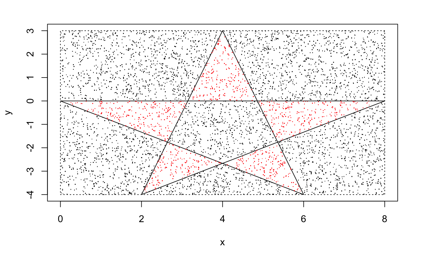
## [1] 11.9504Now we can write the point in polygon function with both algorithm:
point_inside_v2 <- function(x,y,x0,y0, method = "wind") {
  if (method == "wind") {
    wind <- winding_number(x,y,x0,y0)
    if (wind != 0) return (1) else return(0)
  }
  else if (method == "ray") {
    ray <- ray_pass(x,y,x0,y0)
    if (ray %% 2 == 1) return (1) else return(0)
  }
}
The default algorithm is the winding number.
We can use the new point in polygon function to reconstruct the function of the Monte Carlo Method.
area_mc_method_v3 <- function(x,y,k=5000, plotpoly=TRUE, method = "wind") {
  if (length(x) <= 2) return("Input values are not vaild. Error: Only two vertices")
  type <- type_of_polygon_v2(x,y)
  if (type == "Convex") {
    print("Convex Polygon")
  } else if (type == "Self-intersecting") {
    print("Self-intersecting Polygon")
  } else if (type == "Concave") {
    print("Concave Polygon")
  }
  count <- 0
  rectangle_area <- (max(x)-min(x))*(max(y)-min(y))
  random_x <- generate_k_random_point(x,y,k)$x
  random_y <- generate_k_random_point(x,y,k)$y
  inside <- c()
  for (i in 1:k) {
    count <- count + point_inside_v2(x,y,random_x[i],random_y[i],method)
    if (point_inside_v2(x,y,random_x[i],random_y[i],method) == 1) inside <- c(inside, i)
  }
  approximate_area <- count/k*rectangle_area
  if (plotpoly) {
    plot(x,y,pch="")
    polygon(x,y)
    polygon(c(min(x), max(x), max(x), min(x)), c(min(y), min(y), max(y), max(y)), lty = 3)
    points(random_x[inside],random_y[inside], pch = ".", col = "red")
    points(random_x[-inside],random_y[-inside], pch = ".")
  }
  return(approximate_area)
}
In theory, the version 3 should work very well: it's much faster than the obese version 2n, less error and works on almost all polygons.
The next section is Monte Carlo Part 3, we will talk more about the Monte Carlo integration.
© Group 18