First of all, it is not easy to apply Monte Carlo method to all kind of polygons. Therefore we need to identify what is the type of the given polygon before we apply the Monte Carlo method. As the main research topic is to estimate the area of a convex polygon, the start point is to think about how to classify the convex and non-convex polygon in R.
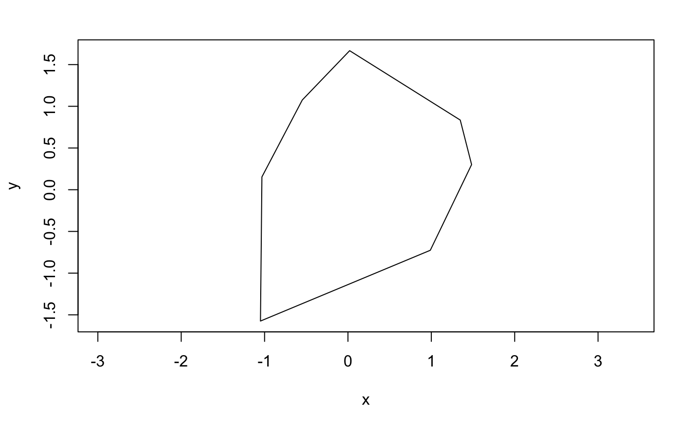
Figure 2.1 is a random generated convex octagon with all interior angles are less than $\frac{\pi}{2}$.
But before we start, it is noticeable that any triangle is convex. As the sum of the interior angles of a triangle is $\frac{\pi}{2}$, all three angles should less than $\frac{\pi}{2}$ rad, which means it is a convex polygon.
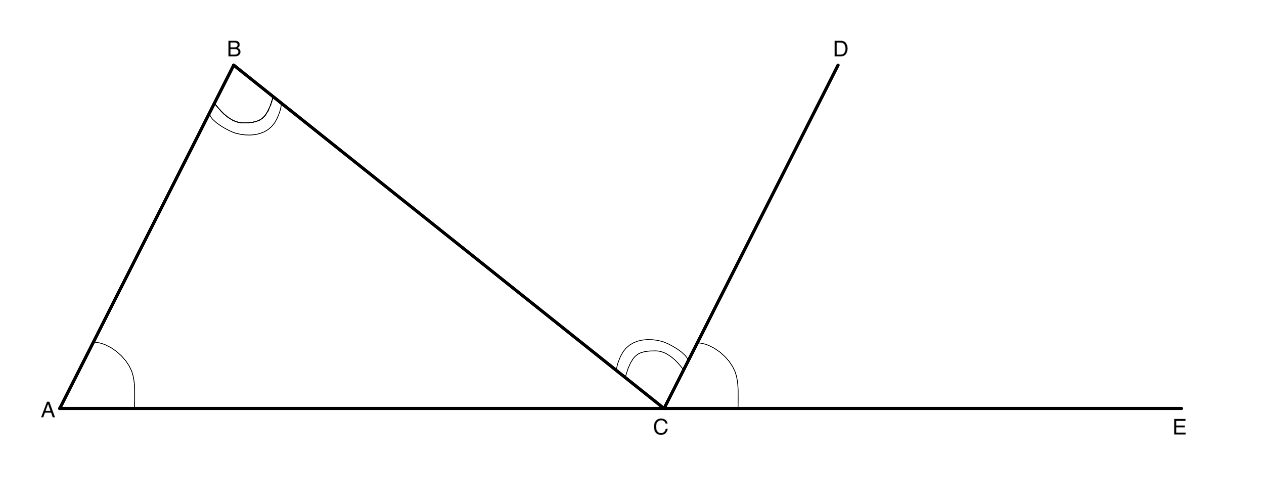
For a triangle $ABC$, if we plot a line parallels to the line $AB$ and passes through vertex $C$ and point $D$, extend line $AC$ to point $E$, as shown in Figure 2.2. Then $\angle{BAC}$ has the same size as $\angle{DCE}$, $\angle{ABC}$ has the same size as $\angle{BCD}$. It is easy to show that $\angle{DCE} + \angle{BCD} + \angle{BCA} = \pi$, since $A$,$C$ and $E$ are in the same line, and a straight angle is $\pi$.
Furthermore, it is also easy to show that the sum of interior angles of a $n$-side simple polygon is $(n-2)\pi$, as we can divide the simple polygon into many triangles. For example:
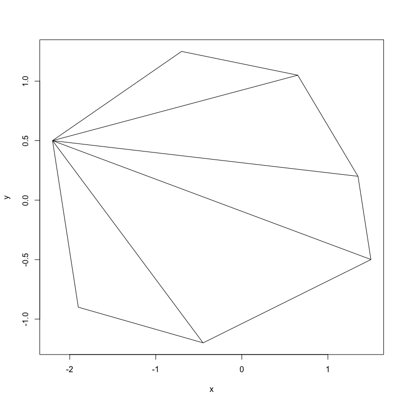
It is obvious that the sum of the interior angles of the octagon is the same as the sum of the interior angles of six triangles.
Starting from any vertex of a convex polygon, there exists $n-3$ vertices are unconnected to it. If $n-3$ diagonals are drawn from the vertex, then the polygon can be decomposed into $n-2$ triangles, which means the sum of the interior angles of the convex polygon is $(n-2)\pi$. This process is also known as fan triangulation.[2]
For concave polygon, the formula also works. Also, the sum of angles of the $n$-side self-intersecting polygon is less or equal to $(n-2)\pi$.[3]
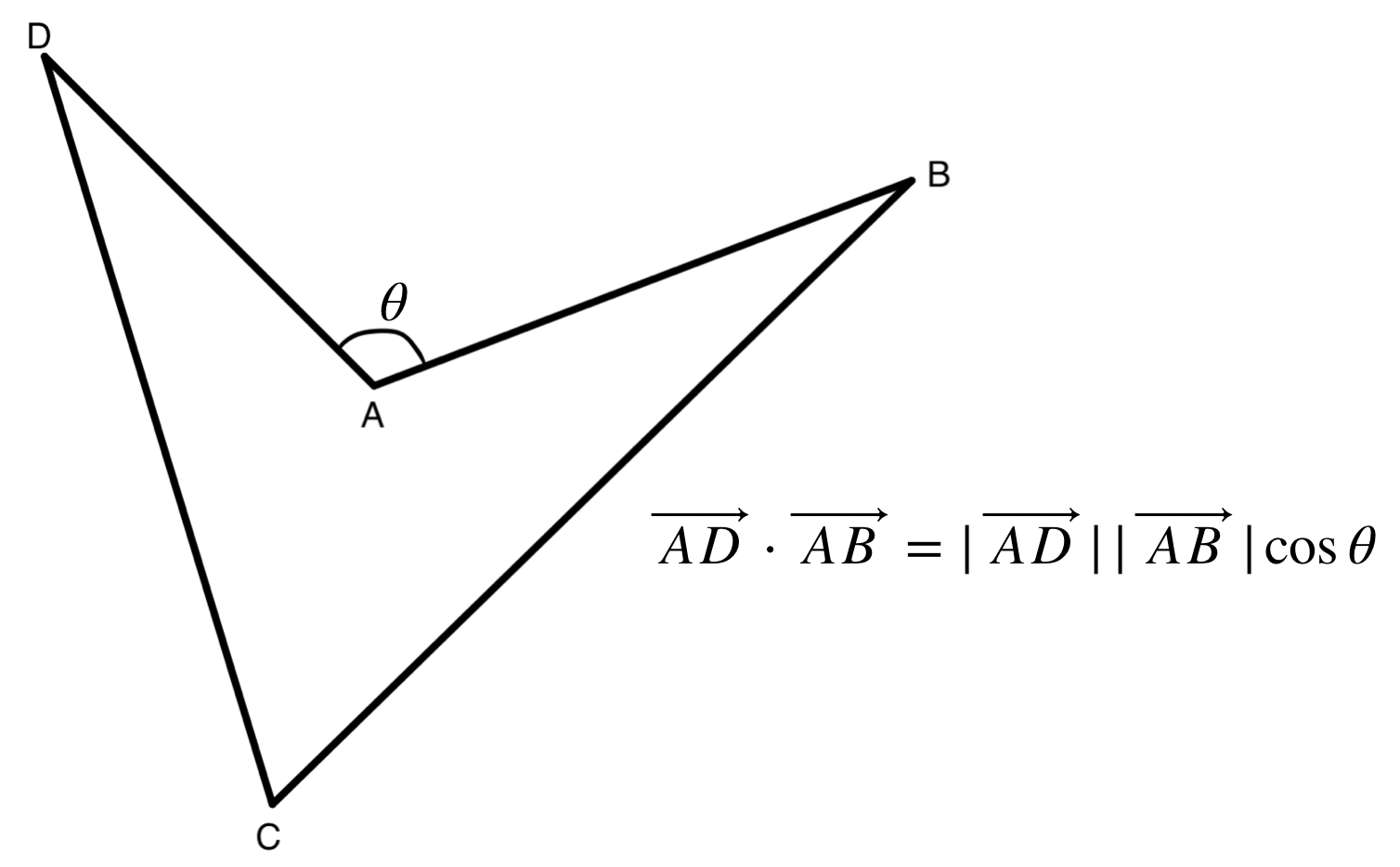
In mathematics, the scalar product or dot product, can be defined for two vectors $\mathbf{u}$ and $\mathbf{v}$ by $$\mathbf{u} \cdot \mathbf{v}=|\mathbf{u}||\mathbf{v}|\cos{\theta},$$ where $\theta$ is the angle between $\mathbf{u}$ and $\mathbf{v}$, and $|\mathbf{u}|$ is the magnitude of itself.
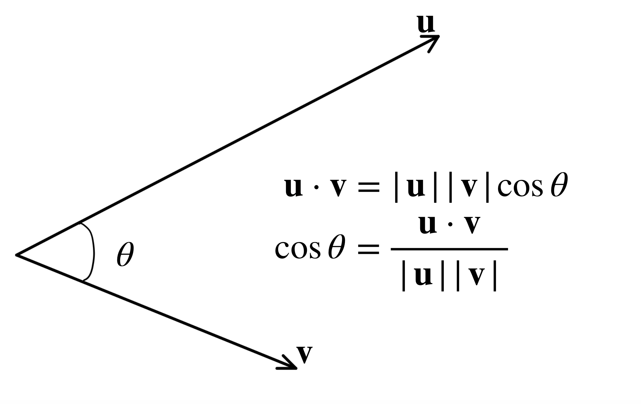
The angle between two vectors can be determined by scalar product, by arranging the formula: $$\cos{\theta} = \frac{\mathbf{u} \cdot \mathbf{v}}{|\mathbf{u}||\mathbf{v}|},$$ and apply the inverse cosine, $$\theta = \arccos{\bigg(\frac{\mathbf{u} \cdot \mathbf{v}}{|\mathbf{u}||\mathbf{v}|}\bigg)}.$$
In a concave polygon, there exists at least one interior angle is more than $\frac{\pi}{2}$. But if we use the above formula to find out the angle $\theta$ larger than $\pi$, it will return $2\pi-\theta$. As $\cos{(2\pi-\theta)} = \cos{\theta}$, and the inverse cosine always return the smallest value of $\theta$.
By scalar product, all angles of the polygon can be determined. But as Figure 2.5 shown, if the method is applied to concave polygon, then there might be some exterior angles calculated. The sum of the angles should be less than $\frac{\pi}{2}$ in this case. Hence it is possible to identify the type of a polygon with the scalar product: If the sum of the angles equals to $\frac{\pi}{2}$, then it is Convex; else it is Non-convex.
Now convert the algorithm into a function:
type_of_polygon <- function(x,y) {
  n <- length(x)
  direction <- list()
  angle <- c()
  convex <- FALSE
  x[n+1] <- x[1]
  y[n+1] <- y[1]
  if (n < 3) return("Error: Please enter more than three points")
  if (n == 3) return("Convex")
  for (i in 1:n) {
    direction <- c(direction,list((c(x[i+1],y[i+1]) - c(x[i],y[i])))) ## Direction of the lines
  }
  direction[n+1] <- direction[1]
  for (i in 1:n) {
    dotproduct <- direction[[i]] %*% (-1*direction[[i+1]])
    nomproduct <- norm(direction[[i]])*norm(-1*direction[[i+1]])
    angle <- c(angle,acos(dotproduct/nomproduct))
  }
  if ((n-2)*pi - sum(angle) > 2.11e-08) { # Due to precision of double
    convex <- FALSE
  } else if ((n-2)*pi - sum(angle) <= 2.11e-08) {
    convex <- TRUE
  }
  if (convex) {
    return("Convex")
  } else {
    return("Non-convex")
  }
}
For a polygon with more than 3 sides, this function will calculate the directions from the first vertex to the second vertex, the second to the third and so on. But to calculate the right angle, the second direction vector should change the direction, like -1*direction[[i+1]]. For example:
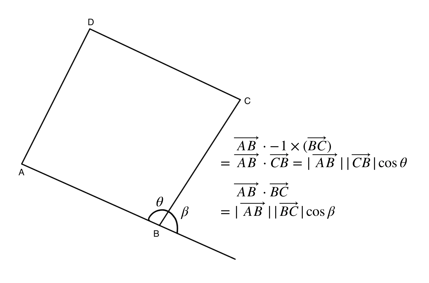
As shown in Figure 2.6, the reason of why the second direction vector needs to be changed the direction is to get the right angle.
The sum of the angles is determined, then if the sum is less than $\frac{\pi}{2}$, the polygon is not convex. Else, it is convex.
For the Non-convex polygon, the situation is more complex. But now we can use the type_of_polygon function to identify the convex polygon first, and start to classify the non-convex polygon. There are only two left, which are concave and self-intersecting polygons.
One possible way to achieve this is, if a non-convex polygon is self-intersected, then there exists at least one point of intersection which is not the vertex of the polygon. Therefore we can write a function to determine that, if two non-adjacent edges have at least one point of intersection, then the polygon is self-intersected. Else, it is concave.
In order to do that, the best way is to write a function that can return the line equations of the edges of the given polygon first, then test each line equations with each other expect the adjacent one. So let's start to do that:
line_equ <- function(x,y) {
  fx <- c()
  grad <- gradient(x,y)
  n <- length(x)
  f <- function(i) {
    g <- grad[i] # We can avoid to use the case when gradient is Inf or -Inf
    xm <- x[i]
    ym <- y[i]
    function(x) g*(x - xm) + ym
  }
  for (i in 1:n) { #  In case input the same vertex twice or more
    if (is.nan(grad[i])) {
      return(cat("Input values are not vaild, repeat points detected."))
    }
    fx <- c(fx,f(i))
  }
  return(fx)
}
Line equation by the gradient $m$ and a point $(x_0,y_0)$ is $y - y_0 = m(x - x_0)$, or $y = m(x - x_0) + y_0$.
The function above will not work if gradient between two points can not be deteremined, like gradient between the two exactly same points. Also if the g radient is Inf or -Inf, then this function will only return Inf or -Inf. But it is possible to avoid that in the later function.
Also, it is better to add another function that in case the request of non-exist line equation happens. Like the request to find the zeroth or $(n+1)$th line equation of the edge of the $n$-side polygon.
linen_equ <- function(x,y,n) {
  if(n == 0) {
    return(line_equ(x,y)[[length(x)]])
  } else if (n > length(x)) {
    n1 <- n %% length(x)
    return(line_equ(x,y)[[n1]])
  } else {
    return(line_equ(x,y)[[n]])
  }
}
Now convert the algorithm of how to identify the concave or self-intersecting polygon into a function:
type_of_polygon_v2 <- function(x,y) {
  if (type_of_polygon(x,y) == "Convex") return("Convex") else
  xv2 <- x # So x[n+1] <- x[1] will not affect the initial x-coordinate of vertices
  s <- 0
  n <- length(x)
  x[n+1] <- x[1]
  for (i in 1:n) {
    if (i == 1) {
      for (j in (1:n)[-c(1,2,n)]) {
        if (abs(x[1] - x[2]) < 0.1) { # Mostly when gradient is Inf or -Inf happens
          if (abs(x[j] - x[j+1]) < 0.01) break
          if (linen_equ(xv2,y,j)(x[1]) <= max(y[1],y[2]) && linen_equ(xv2,y,j)(x[1]) >= min(y[1],y[2])) {
            s <- s + 1
            break
          }
        } else for (k in seq(x[1],x[2],length.out=101)) {
           if (is.na(abs(linen_equ(xv2,y,1)(k) - linen_equ(xv2,y,j)(k)))) next
           if (abs(linen_equ(xv2,y,1)(k) - linen_equ(xv2,y,j)(k)) < 0.1 ) {
             xi <- k
             if (xi <= max(x[j],x[j+1]) && xi >= min(x[j],x[j+1])) {
              s <- s + 1
              break
            }
           }
         }
      }
    } else if (i == n) {
      for (j in (1:n)[-c(1,(n-1),n)]) {
        if (abs(x[1] - x[n]) < 0.1) {
          if (abs(x[j] - x[j+1]) < 0.01) break
          if (linen_equ(xv2,y,j)(x[1]) <= max(y[1],y[n]) && linen_equ(xv2,y,j)(x[1]) >= min(y[1],y[n])) {
            s <- s + 1
            break
          }
        } else for (k in seq(x[n],x[1],length.out=101)) {
          if (is.na(abs(linen_equ(xv2,y,n)(k) - linen_equ(xv2,y,j)(k)))) next
          if (abs(linen_equ(xv2,y,n)(k) - linen_equ(xv2,y,j)(k)) < 0.1 ) {
            xi <- k
            if (xi <= max(x[j],x[j+1]) && xi >= min(x[j],x[j+1])) {
              s <- s + 1
              break
            }
          }
        }
      }
    } else {
      for (j in (1:n)[-c(i-1,i,i+1)]) {
        if (abs(x[i] - x[i+1]) < 0.1) {
          if (abs(x[j] - x[j+1]) < 0.01) break
          if (linen_equ(xv2,y,j)(x[i]) <= max(y[i],y[i+1]) && linen_equ(xv2,y,j)(x[i]) >= min(y[i],y[i+1])) {
            s <- s + 1
            break
          }
        } else for (k in seq(x[i],x[i+1],length.out=101)) {
          if (is.na(abs(linen_equ(xv2,y,i)(k) - linen_equ(xv2,y,j)(k)))) next
          if (abs(linen_equ(xv2,y,i)(k) - linen_equ(xv2,y,j)(k)) < 0.1 ) {
            xi <- k
            if (xi <= max(x[j],x[j+1]) && xi >= min(x[j],x[j+1])) {
              s <- s + 1
              break
            }
          }
        }
      }
    }
  }
  if (s == 0) {
    return("Concave")
  } else {
    return("Self-intersecting")
  }
}
This is a utility function, and will be used in the rest of the project many times.
The key point is to compare each line with the line not next to it. If intersection detects, then it is a self-intersecting polygon. But there are some cases that causes the function to return the incorrect result, like this one:
Or this one:
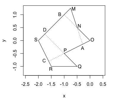
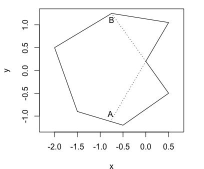
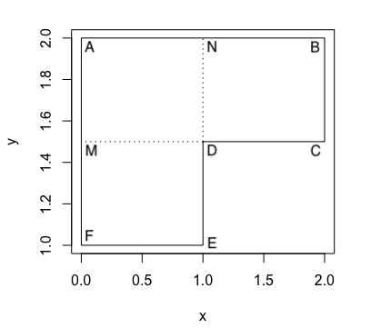
In Figure 2.8, edge $MN$ and $OP$ are not intersected, but line $MN$ and $OP$ intersect at $A$. Even the domain of the line equation is limited by the start point and the end point, it is still possible to return error. For example, the domain of edge $MN$ is inside the domain of the edge $OP$.
To avoid this happens, one possible technique is when a intersection point is detected in the domain of one edge, automatically check it in the domain of another edge. If the intersection point is inside both domains, then the polygon is really the self-intersecting one.
Because this function use linen_equ function, if there exists an edge with gradient is too large or infinity, then type_of_polygon_v2 function will calculate the lower and upper bound of such edge, and use those as limits instead.
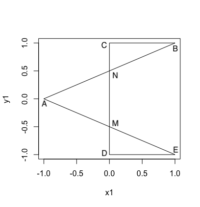
In Figure 2.9, gradient of the line $CD$ is infinity, then the function will only compare the line $CD$ with the line $AB$ and $DE$ at $x=0$ for $-1 \leq y \leq 1$.
What happens if the line needs to be compared with is with large gradient? They should never intersect, so no need to compare them. Like this one:
Compare line $DE$ and $BC$ is not required, so use break to stop that in the function.
The next section is Monte Carlo (Part 1), it is all about the upper and lower bounds of the polygon. A much better approach and be found in the Part 2.
© Group 18