In a plane, a closed curve is a curve with no endpoints and which completely encloses an area.[8][9] If the curve $C$ is formed by a number of line segments, then it is also can be called as polygon. Area of polygon can be considered as the double integral of $1$ over the region of polygon $D$, and by Green's theorem[11] $$\oint_Cf \ dx+g \ dy=\iint_D\left(\frac{\partial g}{\partial x}-\frac{\partial f}{\partial y}\right)dA.$$ We want the right hand side $\frac{\partial g}{\partial x}-\frac{\partial f}{\partial y}$ to be $1$, so let $g(x,y)=x$ and $ \ f(x,y)=0$, then $$A = \oint_Cx \ dy.$$ Which is the line integral on a closed curve $C$. In our case, $C$ is the line segments that form the polygon.
If we can break the curve $C$ into many pieces of segments $C_1, C_2, ..., C_n,$ since the integration has the additive properties over a continuous region, then we have $$\oint_Cx \ dy = \int_{C_1}x \ dy + \int_{C_2}x \ dy + ... + \int_{C_n}x \ dy.$$
In the case of polygon, each segments is the edge of the polygon, then we can find out the line equation of $C_i$ in vector form, which is the $i$-th edge of the polygon. Assume that the coordinates of the $i$-th vertex is $(x_i,y_i)$, then $$\mathbf{r} = \begin{pmatrix} x_i \\ y_i \end{pmatrix} + t\begin{pmatrix} x_{i+1}-x_i \\ y_{i+1}-y_i \end{pmatrix},$$ where $t$ is the parameter and $0 \leq t \leq 1$.
Then we can see $x(t) = x_i + t\ (x_{i+1}-x_i)$ and $y(t) = y_i + t\ (y_{i+1}-y_i)$.
By line integral, $$\oint_{C_i}x \ dy= \int_{0}^{1} (x_i + t\ (x_{i+1}-x_i)) \ \frac{dy}{dt} \ dt = \int_{0}^{1} (t\ (x_{i+1}-x_i) + x_i)(y_{i+1}-y_i) \ dt = \frac{(x_{i+1}+x_i)(y_{i+1}-y_i)}{2}.$$ Hence $$A = \oint_Cx \ dy = \sum_{i=1}^{n} \frac{(x_{i+1}+x_i)(y_{i+1}-y_i)}{2} =\frac{1}{2} \sum_{i=1}^{n} \det\begin{pmatrix} x_i & x_{i+1} \\ y_i & y_{i+1} \end{pmatrix} $$ where $x_{n+1}:= x_1$, $y_{n+1}:=y_1$.
Notice that this is also the formula we used in the mini project 2. Also, this formula is not always working with the self-intersecting polygon.
This formula is widely known as Shoelace formula or Surveyor's area formula[10], it is a special case of the Green's theorem. Apart from using the Green's theorem, there are many ways to get this formula, but using the Green's theorem is one of the easiest ways to get this formula.
Instead of using Shoelace formula, we can also apply the Monte Carlo method to estimate the area of the polygon. Although it is not as fast as Shoelace formula for simple polygon, as it requires to generate a number of points, it can be used to estimate all kind of polygons, including the self-intersecting one. As the only thing we need to know is, whether a point is inside the polygon or not. If there is a suitable algorithm for all kind of polygons, then we can find the area of them by the Monte Carlo method.
The main research topic of this Group Project, is to use the programming method to check whether a point is inside the polygon or not, and therefore estimate the area of the polygon by Monte Carlo method. Also including Monte Carlo integration, the usage of Pick's Theorem, randomly generate a convex polygon, etc.
The main programming language uses in this project is R and the default unit of angle is radian. Explanation of the code might not always in the code.
For the best experience, it is recommended to set the Math Renderer of the MathJax to Common HTML. Simply just right click the MathJax equation.
If the size of the browser window changes, it is also recommended to refresh the website in order to resize the MathJax equation.
This website also adopt dark mode in macOS Mojave 10.14.4 or higher. If the appearance is already in dark mode, then the website will look dark, else it will look light. The default colour theme is dark, unless the system appearance is in light mode, it will always in dark theme.

Polygon is a flat shape with three or more straight sides, and can be classified by the kind of angles and the convexity:
Monte Carlo method is a kind of algorithms that repeatedly using random sample value to estimate the actual result, and it can be extended to Monte Carlo integration[19], which is a statistical method to estimate the integral.
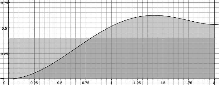
Figure 1.3 shows the function $f(x) = \frac{1}{10}x^{5}-\frac{1}{4}x^{4}-\frac{1}{3}x^{3}+x^{2}$. The integral $\int_{0}^{2} f(x)\ dx$ can be considered as the area under the curve between $[0,2]$. Instead of doing the integration, consider the rectangle that has the same base length and area. We can use the Monte Carlo method to estimate the height of the rectangle, such that the area is approximately the same as the area under the curve.
Let $p(x)$ be a function and we want to find out the area $$\int_{a}^{b} p(x)\ dx.$$ If there is a random variable $X$ with density $f(x)$, then the expected value of $Z = p(X)$ will be $$ E[p(X)] = \int_{-\infty}^{\infty} p(x)f(x)\ dx.$$
If we generate a random sample from the distribution of $X$, then an unbiased estimator of $E[p(X)]$ is the sample mean.
In this case, the expect value will be the height of the rectangle that the area of rectangle is the same as the integral.[14]
Also, if we want to estimate the area $\alpha = \int_{a}^{b} p(x)\ dx$, and $X_1, X_2,...,X_n$ is a uniform $U[a,b]$ distribution sample, then $$\hat{p} = \overline{p(X_n)} =\frac{1}{n} \sum_{i=1}^{n} p(X_i)$$ and $$\hat{\alpha} = (b-a)\ \hat{p}.$$ The unbiased estimate of area $\alpha$ is the area of the rectangle, which is $(b-a)\frac{1}{n} \sum_{i=1}^{n} p(X_i)$.
Example 1.1 If we want to estimate the $\pi$ by the Monte Carlo method, first we uniformly generate a number of points on the square $[0,1]^2$. Which is the same thing as, let $X, Y$ be the coordinate of $x$ and $y$, and they have the i.i.d. uniform distribution $ X, Y \overset{\text{i.i.d.}}{\sim} U[0,1]$.
The probability that a random point is inside the quarter circle is: $$P(\text{point in the quarter circle}) = \frac{\text{area of the quarter circle}}{\text{area of the unit square}} = \frac{\pi}{4}.$$
Therefore, $$\pi = 4\cdot P(\text{point in the quarter circle}).$$
Then we can estimate the probability by the Monte Carlo method, and $\pi$ is four times the estimation.
Below is an example of how to estimate $\pi$ by the Monte Carlo method:
That was also a part of homework of the Lab Class 3.
We count the number of points inside the quarter circle, and estimate $p = P(\text{point in the quarter circle})$ by $$\hat{p}= \frac{\text{number of points in the quarter circle}}{\text{total number of points}},$$ and $\pi$ is four times the estimation.
By the Strong Law of Large Numbers, the estimation converges to the real $p$, which leads to the real $\pi$.
Example 1.2 If we want to estimate the $\pi$ by the Monte Carlo integration, we first estimate the area of a quarter unit circle. Let $X_1, X_2, ... , X_{10000}$ be a uniform $U[0,1]$ distribution sample, then $\hat{\alpha} = \frac{1}{10000} \sum_{i=1}^{n} \sqrt{1-X_i^2}$ and $\hat{\pi} = 4 \cdot \hat{\alpha}$. We can test it with the following code:
Using Monte Carlo integration looks faster and easier, but that's because we can find the upper bound of the quarter circle easily. If we want to apply this method to a random polygon, then it will be a huge challange to determine the bounds, or just impossible to find a good definition.
However, it is still possible to determine to upper and lower bounds of the convex polygon, which will be introduced in the Monte Carlo Part 1.
Generally, to estimate the area of convex polygon, we apply the Monte Carlo method in this way:
If the coordinates of a n-side polygon are $(x_i,y_i)$ where $i=1,2,...,n.$ Then the vertices of the smallest rectangle that enclose the polygon are:
$$(\min(x_i),\min(y_i)), (\max(x_i),\min(y_i)), (\max(x_i),\max(y_i)), (\min(x_i),\max(y_i)).$$
See Figure 1.4.
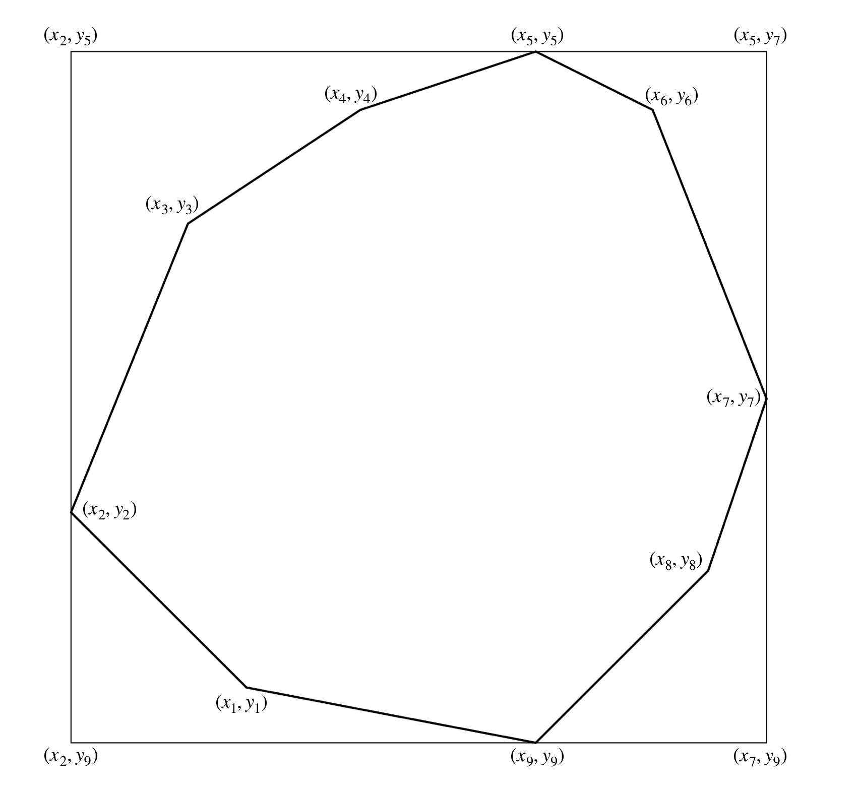
Figure above is a nonagon with rectangle that exactly enclose it.
Then we can apply the Monte Carlo method, uniformly generate same points over the rectangle and so on.
Before next stage, it is better to build some functions first, which will simplify the code later.
norm <- function(x) sqrt(sum(x^2)) # Magnitude of a vector, norn

start_from_miny <- function(x,y) { # Reorder the given value of x and y
  new_x <- c()
  new_y <- c()
  n <- length(x)
  x <- c(x, x)
  y <- c(y, y)
  for (i in 1:n) {
    new_x[i] <- x[match(min(y),y) + i - 1]
    new_y[i] <- y[match(min(y),y) + i - 1]
  }
  return(list(x = new_x, y = new_y)) # It will return a list of two vectors, one is new_x and another is new_y
}

start_from_minx <- function(x,y) { # Reorder the vertices by x position, converse to the above
  new_x <- c()
  new_y <- c()
  n <- length(x)
  x <- c(x, x)
  y <- c(y, y)
  for (i in 1:n) {
    new_x[i] <- x[match(min(x),x) + i - 1]
    new_y[i] <- y[match(min(x),x) + i - 1]
  }
  return(list(x = new_x, y = new_y))
}

anti_rot <- function(x,y) { # Change the rotation order of the given points
  n <- length(x)
  x1 <- x[1]
  y1 <- y[1]
  x1 <- c(x1, rev(x[-1]))
  y1 <- c(y1, rev(y[-1]))
  return(list(x = x1, y = y1))
}

gradient <- function(x,y) {
  grad <- c()
  n <- length(x)
  x[n+1] <- x[1]
  y[n+1] <- y[1]
  for (i in 1:n) {
    grad[i] <- (y[i+1] - y[i])/(x[i+1] - x[i]) # Gradient bewteen any two consecutive points
  }
  return(grad)
}

vector_rot90 <- function(x) {
  return(c(-x[2],x[1]))
}

perpdot <- function(x,y) {
  n <- length(x)
  x[n+1] <- x[1]
  y[n+1] <- y[1]
  direction <- list()
  perpdot <- c()
  for (i in 1:n) {
    direction <- c(direction,list((c(x[i+1],y[i+1]) - c(x[i],y[i]))))
  }
  direction[n+1] <- direction[1]
  for (i in 1:n) {
    perpdotproduct <- vector_rot90(direction[[i]]) %*% direction[[i+1]]
    perpdot <- c(perpdot,perpdotproduct)
  }
  reorder <- c()
  reorder <- c(reorder, perpdot[n])
  reorder <- c(reorder, perpdot[1:(n-1)])
  return(reorder)
}
norn will return the magnitude of a vector x
start_from_miny requires the coordinates of polygon and will return a list with member x and y. Those are the reordered vertices, and the first vertex will have the minimum $y$ coordinate.
start_from_minx is simliar to start_from_miny, the only difference is the first vertex will have the minimum $x$ coordinate.
anti_rot will reverse the order of the vertices
gradient will return the gradient of the edges of the input polygon. i.e. gradient(x,y)[1] is the gradient of the line connected the points (x[1],y[1]) and (x[2],y[2])
vector_rot90 will anticlockwise rotate the input vector $\frac{\pi}{2}$ radians.
perpdot is simliar to gradient, expect it will return the perp dot product of the edge before and the edge after of a vertex. The idea of perp dot product will be introduced later in Monte Carlo (Part 1).
With all the preparations, now we can start to identify the type of polygon.
© Group 18