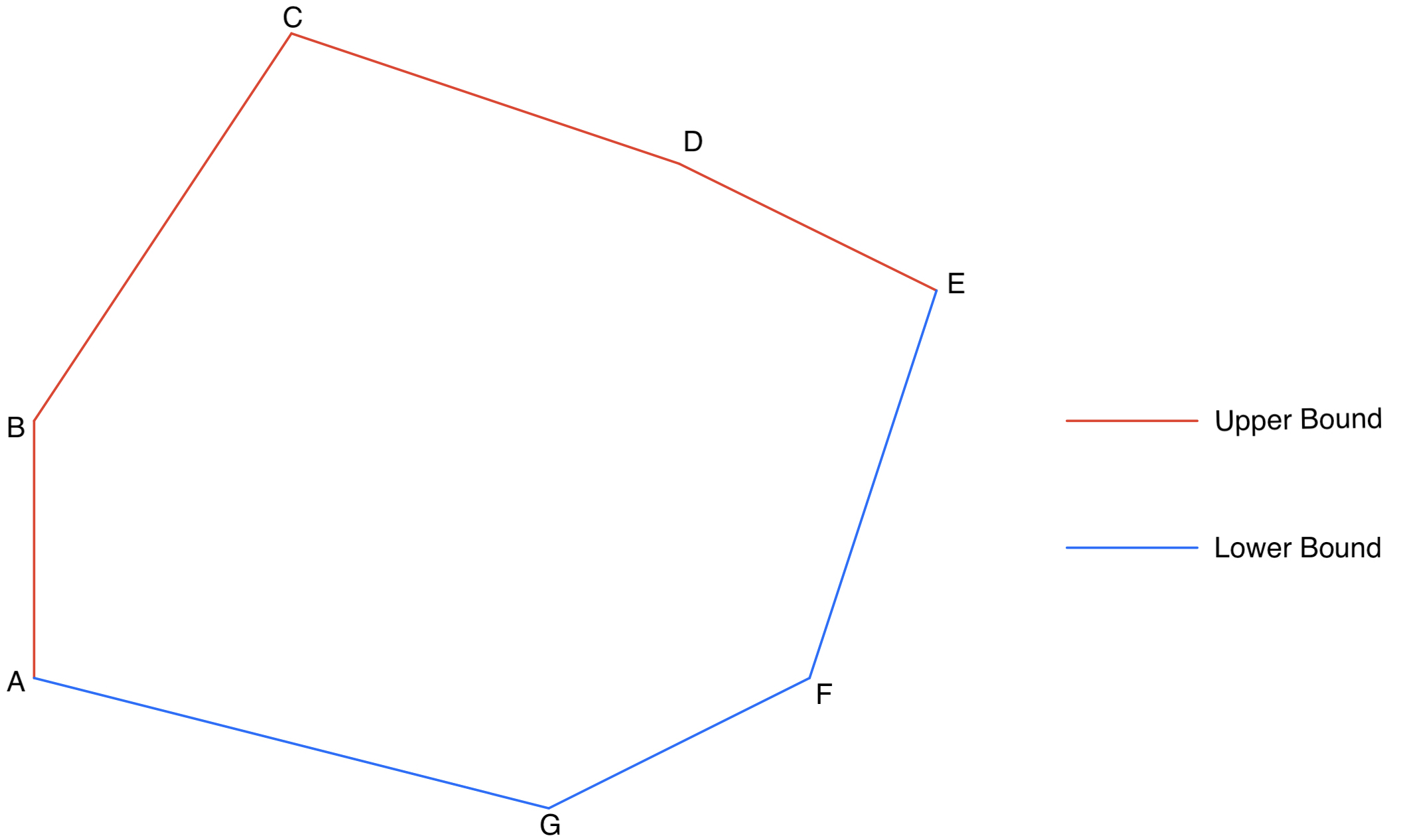
If a point is inside a convex polygon, then there exists an upper bound and a lower bound, and the $y$-coordinate of the point is within the bounds.
In Figure 3.1, red lines indicate the upper bound and blue lines indicate the lower bound. Notice that line $AB$ can be part of both upper bound and lower bound, depends on the order of the coordinates. If start from $A$ and end at $G$, then line $AB$ is the part of upper bound.
Let's summarise it to the definition of the upper and lower vertex.
Definition 3.1 (Upper Vertex) In a convex polygon, starting from the vertex with minimum $x$-coordinate in clockwise direction and ending at the vertex with maximum $x$-coordinate, the vertices in-between are upper vertices.
Definition 3.2 (Lower Vertex) In a convex polygon, starting from the vertex with minimum $x$-coordinate in anticlockwise direction and ending at the vertex with maximum $x$-coordinate, the vertices in-between are lower vertices.
Definition 3.3 (Bounded Vertex) In a convex polygon, if a vertex has the minimum or maximum $x$ value among all vertices, then it is a bounded vertex.
But how the minimum $x$-coordinate to be well-defined if there exists two vertices with the same $x$-coordinate and both are minimum? Like in Figure 3.1, vertex $A$ and vertex $B$ both have the same $x$-coordinate. Then it depends on the order of the vertices.
Now then convert the definiton into a function:
classify <- function(x,y) {
  min_index <- match(min(x),x)
  max_index <- match(max(x),x)
  grad <- gradient(start_from_minx(x,y)$x,start_from_minx(x,y)$y)
  n <- length(x)
  for (i in c(1,n)) {
    if (grad[i] == -Inf) grad[i] <- Inf
  }
  upper_index <- c()
  lower_index <- c()
  bounded_index <- sort(c(min_index,max_index))
  if (grad[1] < grad[n]) {
    if (min_index > max_index) {
      upper_index <- c((max_index+1):(min_index-1))
      if (min_index == n) {
        if (max_index == 1) lower_index <- c(0) else lower_index <- c(1:(max_index-1))
      } else {
        if (max_index == 1) lower_index <- c((min_index+1):n)
        else lower_index <- c(1:(max_index-1),(min_index+1):n)
      }
    } else if (min_index < max_index) {
      lower_index <- c((min_index+1):(max_index-1))
      if (max_index == n) {
        if (min_index == 1) upper_index <- c(0) else upper_index <- c(1:(min_index-1))
      } else {
        if (min_index == 1) upper_index <- c((max_index+1):n)
        else upper_index <- c(1:(min_index-1),(max_index+1):n)
      }
    }
  } else if (grad[1] > grad[n]) {
    if (min_index > max_index) {
      lower_index <- c((max_index+1):(min_index-1))
      if (min_index == n) {
        if (max_index == 1) upper_index <- c(0) else upper_index <- c(1:(max_index-1))
      } else {
        if (max_index == 1) upper_index <- c((min_index+1):n)
        else upper_index <- c(1:(max_index-1),(min_index+1):n)
      }
    } else if (min_index < max_index) {
      upper_index <- c((min_index+1):(max_index-1))
      if (max_index == n) {
        if (min_index == 1) lower_index <- c(0) else lower_index <- c(1:(max_index-1))
      } else if (min_index == 1) lower_index <- c((max_index+1):n)
        else lower_index <- c(1:(min_index-1),(max_index+1):n)
    }
  }
  return(list(ui = upper_index, li = lower_index, bi = bounded_index))
}
If there is no lower vertex or upper vertex, then the function will return 0 instead.
Also, we can now write a function to reorder the vertices, not just start from minimum of $x$, but also in anticlockwise direction.
anticlockwise_order_minx <- function(x,y) {
  n <- length(x)
  grad <- gradient(start_from_minx(x,y)$x,start_from_minx(x,y)$y)
  for (i in c(1,n)) {
    if (grad[i] == -Inf) grad[i] <- Inf
  }
  if (grad[1] < grad[n]) return(list(x = start_from_minx(x,y)$x, y = start_from_minx(x,y)$y))
  if (grad[1] > grad[n]) return(list(x = start_from_minx(rev(x),rev(y))$x, y = start_from_minx(rev(x),rev(y))$y))
}To avoid the error happens in this case, notice that the type of polygon and area will not be affected if only the start point and the end point of the line remained. That means we can remove those vertices first before we apply the other methods.
start_from_minx_v2 <- function(x,y) {
  x1 <- start_from_minx(x,y)$x
  y1 <- start_from_minx(x,y)$y
  n <- length(x)
  index <- c()
  grad <- gradient(x1,y1)
  grad[n+1] <- grad[1]
  for (i in 1:n) {
    if (grad[i] == grad[i+1]) {
      index <- c(index,(i+1))
      repeats <- TRUE
    }
    else repeats <- FALSE
  }
  if (repeats) return(list(x = x1[-index],y = y1[-index])) else return(list(x = x1,y = y1))
}
and combine with the function anticlockwise_order_minx:
anticlockwise_order_minx <- function(x,y) {
  n <- length(x)
  grad <- gradient(start_from_minx_v2(x,y)$x,start_from_minx_v2(x,y)$y)
  for (i in c(1,n)) {
    if (grad[i] == -Inf) grad[i] <- Inf
  }
  if (grad[1] < grad[n]) return(list(x = start_from_minx(x,y)$x, y = start_from_minx(x,y)$y))
  if (grad[1] > grad[n]) return(list(x = start_from_minx(rev(x),rev(y))$x, y = start_from_minx(rev(x),rev(y))$y))
}
But generally, please avoid to enter such polygon.
Now we classify the vertices, and have a function to reorder the polygon in anticlockwise direction and start from minimum $x$. Then we can find the lower and upper bounds. Lower bound of a convex polygon, is a set of the line equations that constructed the lower half of the polygon, starting from the minimum of $x$ to the maximum of $x$. Which is:
lower_bound <- function(x,y,x0) {
  x1 <- anticlockwise_order_minx(x,y)$x
  y1 <- anticlockwise_order_minx(x,y)$y
  x_max <- match(max(x1),x1)
  for (i in 1:(x_max-1)) {
    if (x0 <= x1[i+1] && x0 >= x1[i]) return(linen_equ(x1,y1,i)(x0))
  }
}
Similarly, the upper bound is:
upper_bound <- function(x,y,x0) {
  x2 <- anticlockwise_order_minx(x,y)$x
  y2 <- anticlockwise_order_minx(x,y)$y
  grad <- gradient(x2,y2)
  x_max <- match(max(x2),x2)
  n <- length(x2)
  for (i in x_max:n) {
    if (i == n) {
      if (x0 >= x2[1] && x0 <= x2[n]) {
        if (abs(grad[n]) == Inf) return(y2[n]) else return(linen_equ(x2,y2,n)(x0))
      }
    } else if (i == x_max) {
        if (x0 >= x2[i+1] && x0 <= x2[i]) {
          if(abs(grad[x_max]) == Inf) return(y2[x_max + 1]) else return(linen_equ(x2,y2,i)(x0))
        }
    } else {
      if (x0 >= x2[i+1] && x0 <= x2[i]) {
        return(linen_equ(x2,y2,i)(x0))
      }
    }
  }
}If a point $(x_0,y_0)$ is inside the polygon, then at $x_0$, $y_0$ must between the lower and upper bounds. Hence:
point_inside <- function(x,y,x0,y0) {
  if (x0 < min(x) || x0 > max(x) || y0 < min(y) || y0 > max(y)) return(0)
  if (y0 <= upper_bound(x,y,x0) && y0 >= lower_bound(x,y,x0)) return(1) else return(0)
}
Also the point should inside the circumscribe rectangle, if not then it is not inside the polygon.
If a point is inside the polygon, then the function will return 1, else 0.
Now we can start to randomly generate a number of points, can apply the Monte Carlo method. There is also a function to create the point within the rectangle that exactly cover the polygon:
generate_k_random_point <- function(x,y,k) {
  random_x <- runif(k,min(x), max(x))
  random_y <- runif(k,min(y), max(y))
  return(list(x = random_x, y = random_y))
}
Then apply Monte Carlo method:
area_mc_method <- function(x,y,k = 2000, concave = FALSE, plotpoly = TRUE) { # Special concave as example 4
  if (length(x) <= 2) return("Input values are not vaild. Error: Only two vertices")
  if (concave) {
    type <- type_of_polygon_v2(x,y)
    if (type == "Convex") {
      print("Convex Polygon")
    } else if (type == "Self-intersecting") {
      return("Input values are not vaild. Error: Self-intersecting Polygon")
    } else if (type == "Concave") {
      print("Concave Polygon")
    }
  } else {
    type <- type_of_polygon(x,y)
    if (type == "Convex") {
      print("Convex Polygon")
    } else if (type == "Non-convex") {
      return("Input values are not vaild. Error: Non-convex Polygon")
    }
  }
  count <- 0
  rectangle_area <- (max(x)-min(x))*(max(y)-min(y))
  random_x <- generate_k_random_point(x,y,k)$x
  random_y <- generate_k_random_point(x,y,k)$y
  inside <- c()
  for (i in 1:k) {
    count <- count + point_inside(x,y,random_x[i],random_y[i])
    if (point_inside(x,y,random_x[i],random_y[i]) == 1) inside <- c(inside, i)
  }
  approximate_area <- count/k*rectangle_area
  if (plotpoly) {
    plot(x,y,pch="")
    polygon(x,y)
    polygon(c(min(x), max(x), max(x), min(x)), c(min(y), min(y), max(y), max(y)), lty = 3)
    points(random_x[inside],random_y[inside], pch = ".", col = "red")
    points(random_x[-inside],random_y[-inside], pch = ".")
  }
  return(approximate_area)
}
Actually, some special concave polygon can also find the upper bound and lower bound, like the one in the Example 3.1.
Example 3.1 Compute the area of bounded concave polygon with coordinates $(1,1),(3,4),(4,8),(7,5),(6,3),(4,5)$ by Monte Carlo method with point in polygon method is the bounds algorithm.
xe3 <- c(1,3,4,7,6,4)
ye3 <- c(1,4,8,5,3,5)
area_mc_method(xe3,ye3,concave=TRUE)
## [1] "Concave Polygon"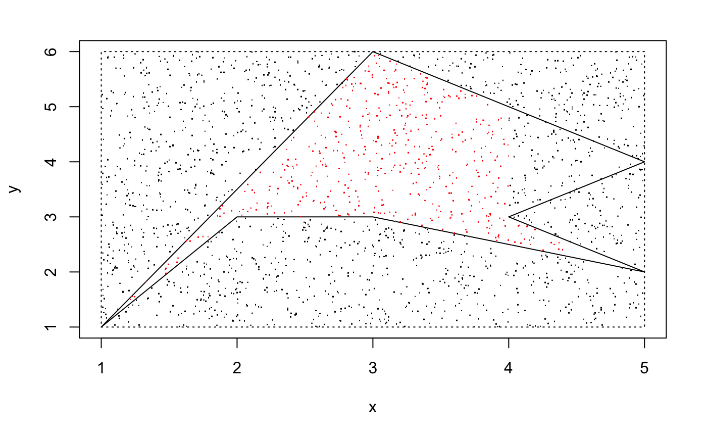
## [1] 9.471That's because both upper and lower bounds can be considered as two functions if it is not one-to-more. If we can not define the bound , the result would be wrong, like the next example.
Example 3.2 Compute the area of the concave polygon with coordinates $(1,1),(3,6),(5,4),(4,3),(5,2),(3,3),(2,3)$ by Monte Carlo method with point in polygon method is the bounds algorithm.
xe5 <- c(1,3,5,4,5,3,2)
ye5 <- c(1,6,4,3,2,3,3)
area_mc_method(xe5,ye5, concave = TRUE) # Wrong result
## [1] "Concave Polygon"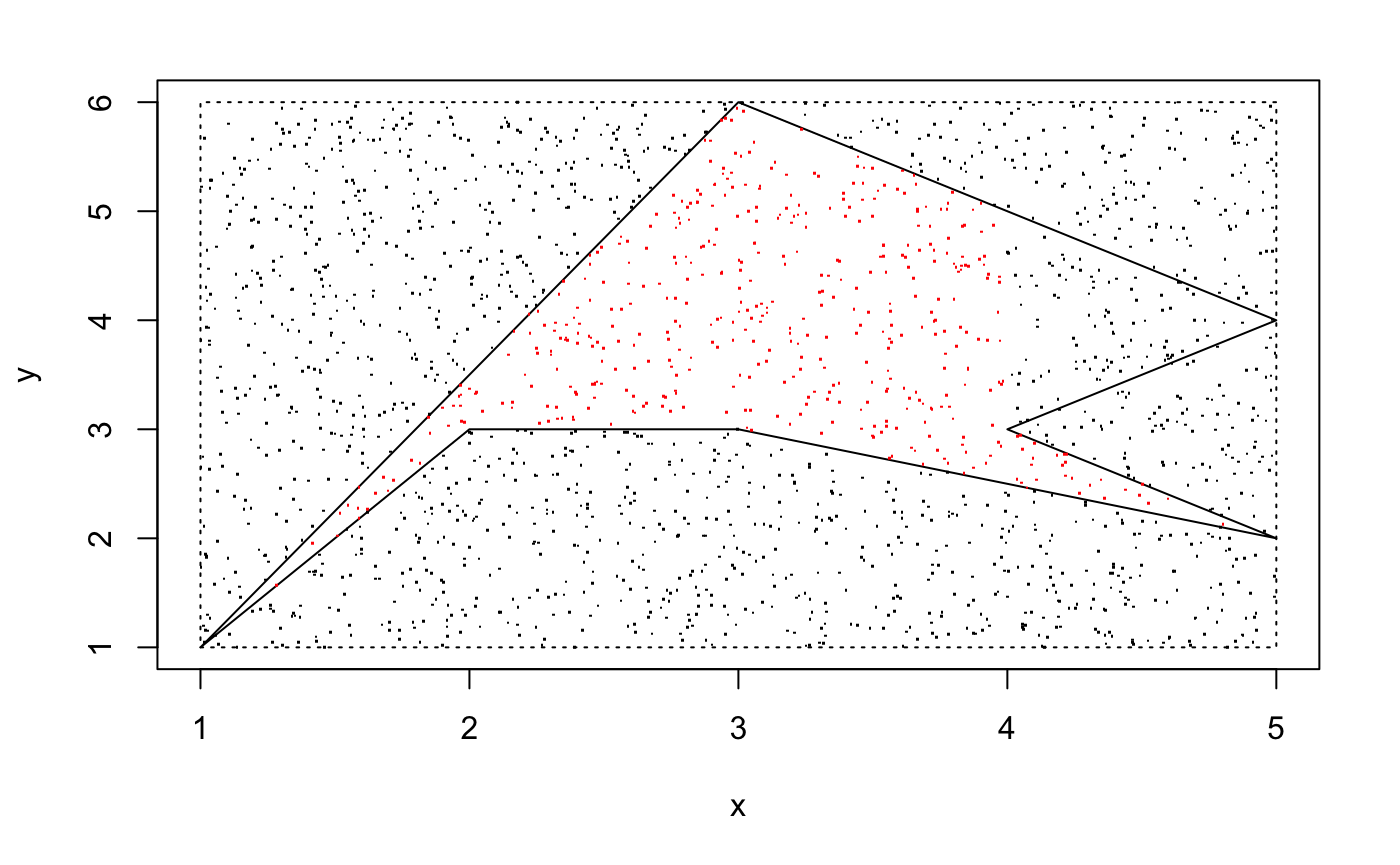
## [1] 4.94The actual area is 6, because the "upper bound" is not a function, so the area_mc_method function ignores some regions.
The area_mc_method function works well for all convex polygon, and some bounded concave polygons.
However, there should be a way to find out the area of all simple polygons, not just some special concave polygons.
Perp Dot Product, or just Perp Product, can be defined for two vectors $\mathbf{u}$ and $\mathbf{v}$ by $$\mathbf{u}\bot\mathbf{v} = \mathbf{u^\bot} \cdot \mathbf{v} = |\mathbf{u}||\mathbf{v}|\sin{\theta},$$ where $\theta$ is the angle between $\mathbf{u}$ and $\mathbf{v}$, and $|\mathbf{u^\bot}|$ is the magnitude. $\mathbf{u^\bot}$ is a vector perpendicular to $\mathbf{u}$, obtained by rotating $\mathbf{u}$ $\frac{\pi}{2}$ rad anticlockwise.[4]
Think about Perp Dot Product in a plane, if $ \begin{align} \mathbf{u} &= \begin{bmatrix} u_{x} \\ u_{y} \end{bmatrix} \end{align}$ then $ \begin{align} \mathbf{u^\bot} &= \begin{bmatrix} 0 & -1 \\ 1 & 0 \end{bmatrix} \begin{bmatrix} u_{x} \\ u_{y} \end{bmatrix} = \begin{bmatrix} - u_{y} \\ u_{x} \end{bmatrix} \end{align}.$ Also if $ \begin{align} \mathbf{v} &= \begin{bmatrix} v_{x} \\ v_{y} \end{bmatrix} \end{align}$ then $$\mathbf{u^\bot} \cdot \mathbf{v} = u_{x}v_{y} - u_{y}v_{x},$$ whereas $$\mathbf{u} \cdot \mathbf{v} = u_{x}v_{x} + u_{y}v_{y}.$$
The scalar projection of $\mathbf{u^\bot}$ in the direction of $\mathbf{v}$ is $|\mathbf{u^\bot}| \sin{\theta} = |\mathbf{u}| \sin{\theta}$, therefore $\mathbf{u^\bot} \cdot \mathbf{v} = |\mathbf{u}||\mathbf{v}|\sin{\theta}$.[1]
The usage of perp dot product in this topic is, if we define the direction vector $\mathbf{v_i}=\mathbf{x_{i+1}}-\mathbf{x_i}$, where $\mathbf{x_i}$ is the vertices of the $n$-side simple polygon, then a simple polygon is convex if and only if $\mathbf{v_i}\bot\mathbf{v_{i+1}}$ has the same sign for all $i$.[5]
WIth this idea, we can also write a function to classify the simple polygon:
type_of_polygon_v3 <- function(x,y) {
  n <- length(x)
  perpd <- perpdot(x,y)
  cp <- 0
  cn <- 0
  for (i in 1:n) {
    if (perpd[i] > 0) cp <- cp + 1 else if (perpd[i] < 0) cn <- cn + 1
  }
  if (cn == n || cp == n) return("Convex") else return("Concave")
}
But it is no better than the version 2, as the polygon must be simple first.
For a concave polygon, there always exists a circumscribe convex polygon that cover the polygon. For example:
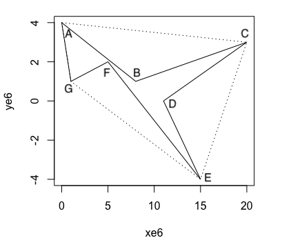
In Figure 3.4, polygon $ACDEG$ is the circumscribe convex polygon of polygon $ABCDEFG$.
Before we start, we can also define the vertices of the simple polygon by the correspoinging angles.[6]
Definition 3.4 (Convex Vertex) For a vertex of the simple polygon, if the angle formed by the two edges at the vertex is less or equal to $\pi/2$, then it is a convex vertex.
Definition 3.5 (Concave Vertex) For a vertex of the simple polygon, if the angle formed by the two edges at the vertex is larger than $\pi/2$, then it is a concave vertex.
Vertices $A,C,D,E,G$ are convex and vertices $B,F$ are concave in Figure 3.4.
The circumscripe convex polygon of the concave polygon, also known as the convex hull of the given points. Convex hull of a set of points $\mathbf{x_i}$ in 2D can be understood as the largest polygon that contain all the points.
One simple way to find the circumscripe polygon, is to connect the convex vertices in the polygon. But sometimes the circumscribe polygon might not be the convex polygon, so we can repeat the process again and again, eventually we will get the circumscribe convex polygon, or the convex hull.
But first, let's classify the vertices:
ang_classify <- function(x,y) {
  n <- length(x)
  if (type_of_polygon(x,y) == "Convex") return(list(convex = 1:n, concave = 0))
  xs <- start_from_minx(x,y)$x
  ys <- start_from_minx(x,y)$y
  perpdot <- perpdot(x,y)
  perpdot_minx <- perpdot(xs,ys)
  cox <- c() # Convex
  coa <- c() # Concave
  gneg <- c()
  gpos <- c()
  if (perpdot_minx[1] < 0) {
    neg_cox <- TRUE
  } else if (perpdot_minx[1] > 0) {
    neg_cox <- FALSE
  }
  for (i in 1:n) {
    if (perpdot[i] < 0) gneg <- c(gneg,i) else if (perpdot[i] > 0) gpos <- c(gpos,i)
  }
  if (neg_cox) {
    cox <- gneg
    coa <- gpos
  } else {
    cox <- gpos
    coa <- gneg
  }
  return(list(convex = sort(cox), concave = sort(coa)))
}
If the type of polygon is convex, then there is no concave vertex.
If there exists $i$ such that the perp dot product of direction vectors $\mathbf{v_i}\bot\mathbf{v_{i+1}}$ has different signs, then the simple polygon is not convex and there exists some concave vertices as there is at least one angle larger than $\frac{\pi}{2}$. Like if a concave polygon have 6 convex vertices and 4 concave vertices, than the perp dot products of the two edges at the convex vertices are either positive or negative, and the perp dot products of the two edges at the concave vertices have the different sign.
So the key problem is, which is positive and which is negative.
Notice that the vertex with minimum of $x$-coordinate should be convex. If not, then it is concave, but there's no vertex with smaller $x$-coordinate than that vertex, which is contradiction. By proof of contradiction, the minimum $x$-coordinate vertex is convex.
The idea is, if the perp dot product of the vertex with minimum $x$ coordinate is negative, then the vertices with negative perp dot product are all convex or vice versa. The function ang_classify uses this idea and it works well.
Since we can classify the convex and concave vertices, now it is the time to find the convex hull of the concave polygon.
outbound_convex_index <- function(x,y) {
  c1c <- ang_classify(x,y)$convex
  while (type_of_polygon(x[c1c],y[c1c]) != "Convex") {
    c1c <- c1c[ang_classify(x[c1c],y[c1c])$convex]
  }
  if (type_of_polygon(x[c1c],y[c1c]) == "Convex") return(c1c)
}
Or a function return the vertices instead of the index of the convex hull:
outbound_convex <- function(x,y) {
  c1c <- ang_classify(x,y)$convex
  while (type_of_polygon(x[c1c],y[c1c]) != "Convex") {
    c1c <- c1c[ang_classify(x[c1c],y[c1c])$convex]
  }
  if (type_of_polygon(x[c1c],y[c1c]) == "Convex") return(list(x = x[c1c],y = y[c1c]))
}
The only problem is, sometimes if the convex vertices are connceted, there could be a self-intersecting polygon. Later there will be a better method to determine a point is in or out, but now assume all the circumscribe polygons are concave or convex.
After we find the index of the convex hull, it is also possible to find the index of the vertices that's not on the convex hull. Just take out the index from 1:n, where n is the number of vertices. So it would be c((1:length(x))[-outbound_convex_index(x,y)]), where x is the $x$-coordinate of the vertices, same as y.
If the first index of the vertices which is not on the convex hull is 1, then we can reorder the vertices and make sure the first one is on the convex hull.
start_from_convex <- function(x,y) {
if (c(1:length(x))[-outbound_convex_index(x,y)][1] == 1) {
order <- c(outbound_convex_index(x,y)[1]:length(x),1:(outbound_convex_index(x,y)[1] - 1))
return(list(x = x[order], y = y[order]))
} else return(list(x = x, y = y))
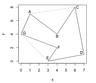
}In Figure 3.5, vertices $B$, $D$ and $F$ are not on the convex hull, as they are not adjacent to each other, there must be three polygons between the convex hull and the polygon $ABCDEFG$, which are $\triangle{ABC}$, $\triangle{CDE}$ and $\triangle{EFG}$. What happens if there exist two or more vertices not on the convex hull? Then they will form a polygon with the vertices next to them on the convex hull. For example:
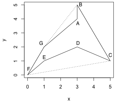
In Figure 3.6, vertices $D$, $E$ are not on the convex hull, and they form a quadrilateral with the nearby vertices $C$ and $F$ which is between the convex hull and the polygon $ABCDEFG$. Also notice that vertex $A$ is not on the convex hull, if we apply the start_from_convex function then the polygon will change the order to $BCDEFGA$.
In the reordered polygon, the index of $A, D$ and $E$ are $7, 3$ and $4$ respectively. Then the polygons bewteen the convex hull and polygon $BCDEFGA$ should have the vertices of index $(6,7,1)$ and $(2,3,4,5)$. Now let's write a function to separate a vector into vectors with consecutive numbers.
sep_vector <- function(x) {
  n <- length(x)
  index <- c()
  sep <- list()
  if (n == 1) {
    sep <- c(sep, list(x))
    return(sep)
  }
  xs <- sort(x)
  xs[n+1] <- xs[1]
  for (i in 1:n) {
    while (xs[i] + 1 == xs[i+1]) {
      i <- i + 1
    }
    index <- c(index,i)
  }
  points <- index[!duplicated(index)]
  m <- length(points)
  sep[1] <- list(xs[1:points[1]])
  for (i in 2:m) {
    sep <- c(sep, list(xs[(points[i-1] + 1):points[i]]))
  }
  return(sep)
}sep_vector(c(1:3,5,8,12,14,16:18,19,24:28,22,21,33:35))## [[1]]
## [1] 1 2 3
##
## [[2]]
## [1] 5
##
## [[3]]
## [1] 8
##
## [[4]]
## [1] 12
##
## [[5]]
## [1] 14
##
## [[6]]
## [1] 16 17 18 19
##
## [[7]]
## [1] 21 22
##
## [[8]]
## [1] 24 25 26 27 28
##
## [[9]]
## [1] 33 34 35If we put c(7,3,4) into the function, output would be a list of c(3,4) and c(7).
Now combine all ideas into this function:
outbound_polygon <- function(x,y) {
  if (type_of_polygon(x,y) == "Convex") return(numeric(0))
  xn <- start_from_convex(x,y)$x
  yn <- start_from_convex(x,y)$y
  n <- length(x)
  sep <- list()
  xl <- list()
  yl <- list()
  polygon_points <- sep_vector(c(1:length(xn))[-outbound_convex_index(xn,yn)])
  xn[n+1] <- xn[1]
  yn[n+1] <- yn[1]
  num_of_polygons <- length(polygon_points)
  for (i in 1:num_of_polygons) {
    centre <- polygon_points[[i]]
    min <- min(centre) - 1
    max <- max(centre) + 1
    sep <- c(sep,list(c(min, centre, max)))
  }
  for (i in 1:num_of_polygons) {
    coord <- sep[[i]]
    xl <- c(xl,list(xn[coord]))
    yl <- c(yl,list(yn[coord]))
  }
  return(list(x = xl, y = yl))
}
The purpose of this funciton is, given the coordinates of the vertices of a concave polygon, it will return the coordinates of the vertices of the polygons bewteen the convex hull of it and itself. Notice that those polygons in-between could also be concave.
Now we can rewrite the area_mc_method function:
area_mc_method_v2 <- function(x,y,k = 2000) {
  if (length(x) <= 2) return("Input values are not vaild. Error: Only two vertices")
  type <- type_of_polygon_v2(x,y)
  if (type == "Convex") {
    print("Convex Polygon")
    return(area_mc_method(x,y,k))
  } else if (type == "Self-intersecting") {
    return("Input values are not vaild. Error: Self-intersecting Polygon")
  } else if (type == "Concave") {
    print("Concave Polygon")
  }
  c1c <- ang_classify(x,y)$convex
  if (type_of_polygon_v2(x[c1c],y[c1c]) == "Self-intersecting") return("Error: Too complex polygon")
  count <- 0
  rectangle_area <- (max(x)-min(x))*(max(y)-min(y))
  random_x <- generate_k_random_point(x,y,k)$x
  random_y <- generate_k_random_point(x,y,k)$y
  x0 <- outbound_convex(x,y)$x
  y0 <- outbound_convex(x,y)$y
  inside <- c()
  for (i in 1:k) {
    count <- count + point_inside(x0,y0,random_x[i],random_y[i])
    if (point_inside(x0,y0,random_x[i],random_y[i]) == 1) inside <- c(inside, i)
  }
  num_of_poly <- length(outbound_polygon(x,y)$x)
  if (num_of_poly != 0) {
    for (j in 1:num_of_poly) {
      xj <- outbound_polygon(x,y)$x[[j]]
      yj <- outbound_polygon(x,y)$y[[j]]
      for (i in 1:k) {
        count <- count - point_inside(xj,yj,random_x[i],random_y[i])
        if (point_inside(xj,yj,random_x[i],random_y[i]) == 1) inside <- inside[inside != i]
      }
    }
  }
  plot(x,y,pch="")
  polygon(x,y)
  polygon(outbound_convex(x,y)$x,outbound_convex(x,y)$y, lty = 3)
  polygon(c(min(x), max(x), max(x), min(x)), c(min(y), min(y), max(y), max(y)), lty = 3)
  points(random_x[inside],random_y[inside], pch = ".", col = "red")
  points(random_x[-inside],random_y[-inside], pch = ".")
  approximate_area <- count/k*rectangle_area
  return(approximate_area)
}
Although it looks very long, inside is very simple: Counting the point inside the convex hull, and remove the point between the convex hull and the polygon. However, if any polygon bewteen the convex hull and the polygon is still concave, then the result will no longer accurate.
Example 3.3 Evaluate the area of the concave polygon with vertices $(1,1),(3,6),(5,4),(4,3),(5,2),(3,3),(2,3)$ by Monte Carlo method.
xe5 <- c(1,3,5,4,5,3,2)
ye5 <- c(1,6,4,3,2,3,3)
area_mc_method(xe5,ye5, concave = TRUE, plotpoly = FALSE)
## [1] "Concave Polygon"## [1] 4.86area_mc_method_v2(xe5,ye5)## [1] "Concave Polygon"## [1] 6.2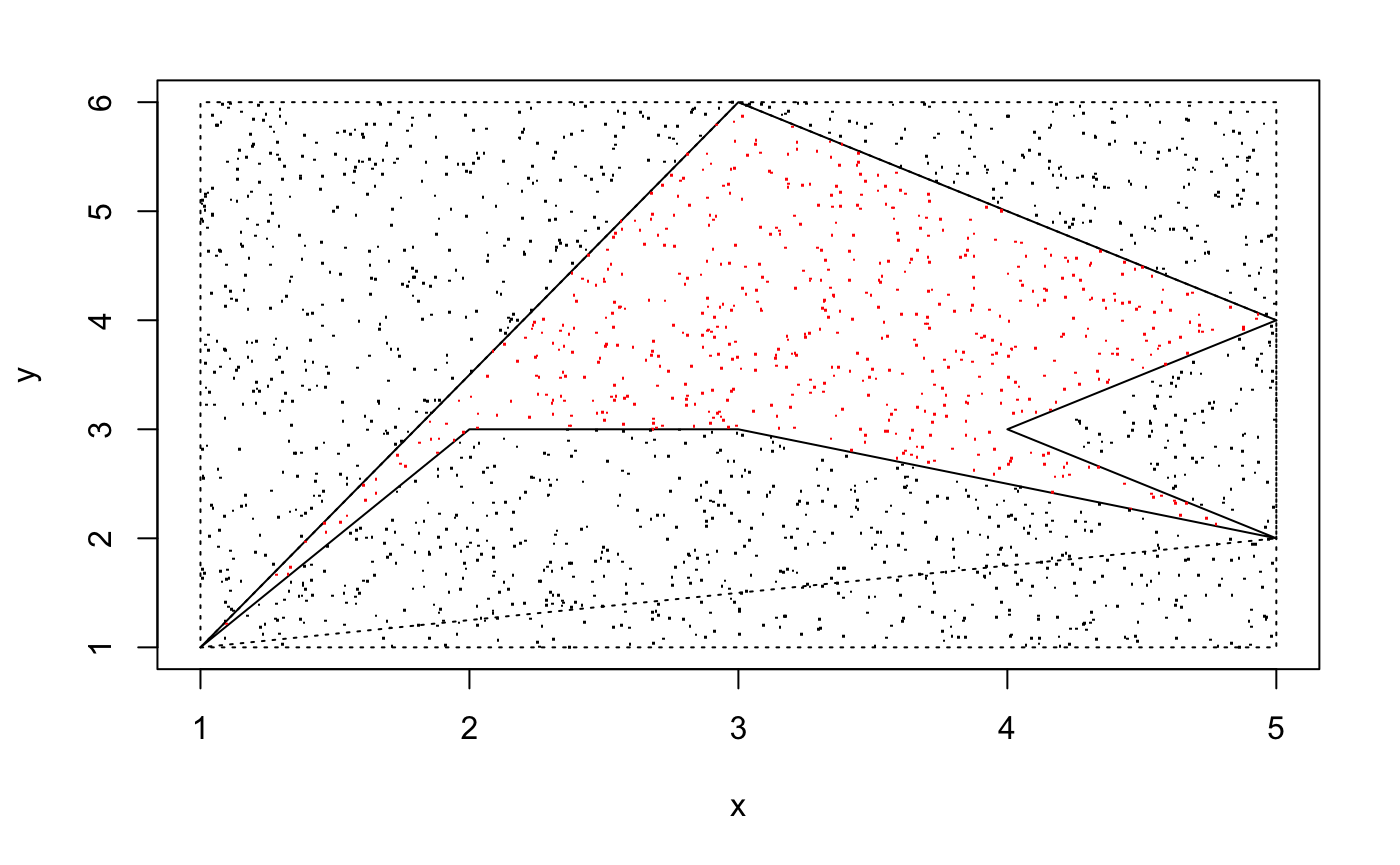
The actural area is 6, so the version 2 return the better approximation. The initial function will miss a part of the polygon, as the "upper bound" is not a function, but we still force it to be a function. When $x \in [4,5]$, the upper bound function will return the smaller $y$, so the point in triangle with vertices $(4,3),(5,4),(4,5)$ will not be counted, and that area is exactly 1.
In area_mc_method_v2 function, we calculate the points inside the convex hull, and then the points in-between and subtract them. If the polygon in-between is concave, then we can do that again: Find the number of points inside the convex hull, subtract the number of points in-between. After that, if there are still some concave polygons left, the size of area would be insignificant compare to the whole polygon, so no need to repeat the process again and again.
Now think about the Taylor series $$f(x)=\sum_{k=0}^\infty f^{(k)}(a)\frac{(x-a)^k}{k!}.$$ If $x-a$ is small, the value of $\frac{(x-a)^k}{k!}$ is insignificant. Hence $$f(x)\approx\ f(a) + f'(a)(x-a)$$ when $x-a$ is small.
Using the same idea, and rewrite the area_mc_method_v2:
area_mc_method_v2n <- function(x,y,k = 2000) {
  if (length(x) <= 2) return("Input values are not vaild. Error: Only two vertices")
  type <- type_of_polygon_v2(x,y)
  if (type == "Convex") {
    print("Convex Polygon")
    return(area_mc_method(x,y,k))
  } else if (type == "Self-intersecting") {
    return("Input values are not vaild. Error: Self-intersecting Polygon")
  } else if (type == "Concave") {
    print("Concave Polygon")
  }
  c1c <- ang_classify(x,y)$convex
  if (type_of_polygon_v2(x[c1c],y[c1c]) == "Self-intersecting") return("Error: Too complex polygon")
  count <- 0
  rectangle_area <- (max(x)-min(x))*(max(y)-min(y))
  random_x <- generate_k_random_point(x,y,k)$x
  random_y <- generate_k_random_point(x,y,k)$y
  x0 <- outbound_convex(x,y)$x
  y0 <- outbound_convex(x,y)$y
  inside <- c()
  for (i in 1:k) {
    count <- count + point_inside(x0,y0,random_x[i],random_y[i])
    if (point_inside(x0,y0,random_x[i],random_y[i]) == 1) inside <- c(inside, i)
  }
  num_of_poly <- length(outbound_polygon(x,y)$x)
  xnc <- list()
  ync <- list()
  if (num_of_poly != 0) {
    for (j in 1:num_of_poly) {
      x1 <- outbound_polygon(x,y)$x[[j]]
      y1 <- outbound_polygon(x,y)$y[[j]]
      if (type_of_polygon(x1,y1) != "Convex") {
         xnc <- c(xnc, outbound_polygon(x1,y1)$x)
         ync <- c(ync, outbound_polygon(x1,y1)$y)
      }
    }
    for (j in (1:num_of_poly)) {
      xj <- outbound_polygon(x,y)$x[[j]]
      yj <- outbound_polygon(x,y)$y[[j]]
      if (type_of_polygon(xj,yj) == "Convex") {
        for (i in 1:k) {
          count <- count - point_inside(xj,yj,random_x[i],random_y[i])
          if (point_inside(xj,yj,random_x[i],random_y[i]) == 1) inside <- inside[inside != i]
        }
      } else {
        xk <- outbound_convex(xj,yj)$x
        yk <- outbound_convex(xj,yj)$y
        for (i in 1:k) {
          count <- count - point_inside(xk,yk,random_x[i],random_y[i])
          if (point_inside(xk,yk,random_x[i],random_y[i]) == 1) inside <- inside[inside != i]
        }
      }
    }
    if (length(xnc) != 0) for (j in 1:length(xnc)) {
      xj <- xnc[[j]]
      yj <- ync[[j]]
      for (i in 1:k) {
        count <- count + point_inside(xj,yj,random_x[i],random_y[i])
        if (point_inside(xj,yj,random_x[i],random_y[i]) == 1) inside <- c(inside, i)
      }
    }
  }
  plot(x,y,pch="")
  polygon(x,y)
  polygon(outbound_convex(x,y)$x,outbound_convex(x,y)$y, lty = 3)
  polygon(c(min(x), max(x), max(x), min(x)), c(min(y), min(y), max(y), max(y)), lty = 3)
  points(random_x[inside],random_y[inside], pch = ".", col = "red")
  points(random_x[-inside],random_y[-inside], pch = ".")
  approximate_area <- count/k*rectangle_area
  return(approximate_area)
}
Example 3.4 Evaluate the area of the concave polygon with vertices xe7 <- c(5,4,7,6,5,6,6,3,4,5,3,2,3,1,3,2), ye7 <- c(4,2,3,-1,1,0,2,1,1,-1,0,1,2,1,3,4) by Monte Carlo method.
xe7 <- c(5,4,7,6,5,6,6,3,4,5,3,2,3,1,3,2)
ye7 <- c(4,2,3,-1,1,0,2,1,1,-1,0,1,2,1,3,4)
area_mc_method_v2(xe7,ye7)
## [1] "Concave Polygon"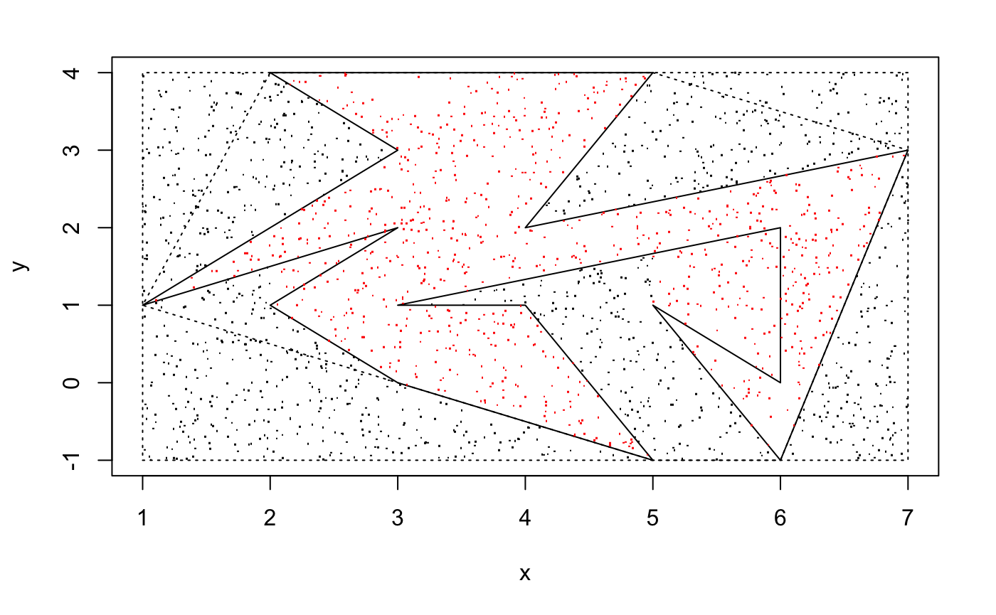
## [1] 13.59xe7 <- c(5,4,7,6,5,6,6,3,4,5,3,2,3,1,3,2)
ye7 <- c(4,2,3,-1,1,0,2,1,1,-1,0,1,2,1,3,4)
area_mc_method_v2n(xe7,ye7)## [1] "Concave Polygon"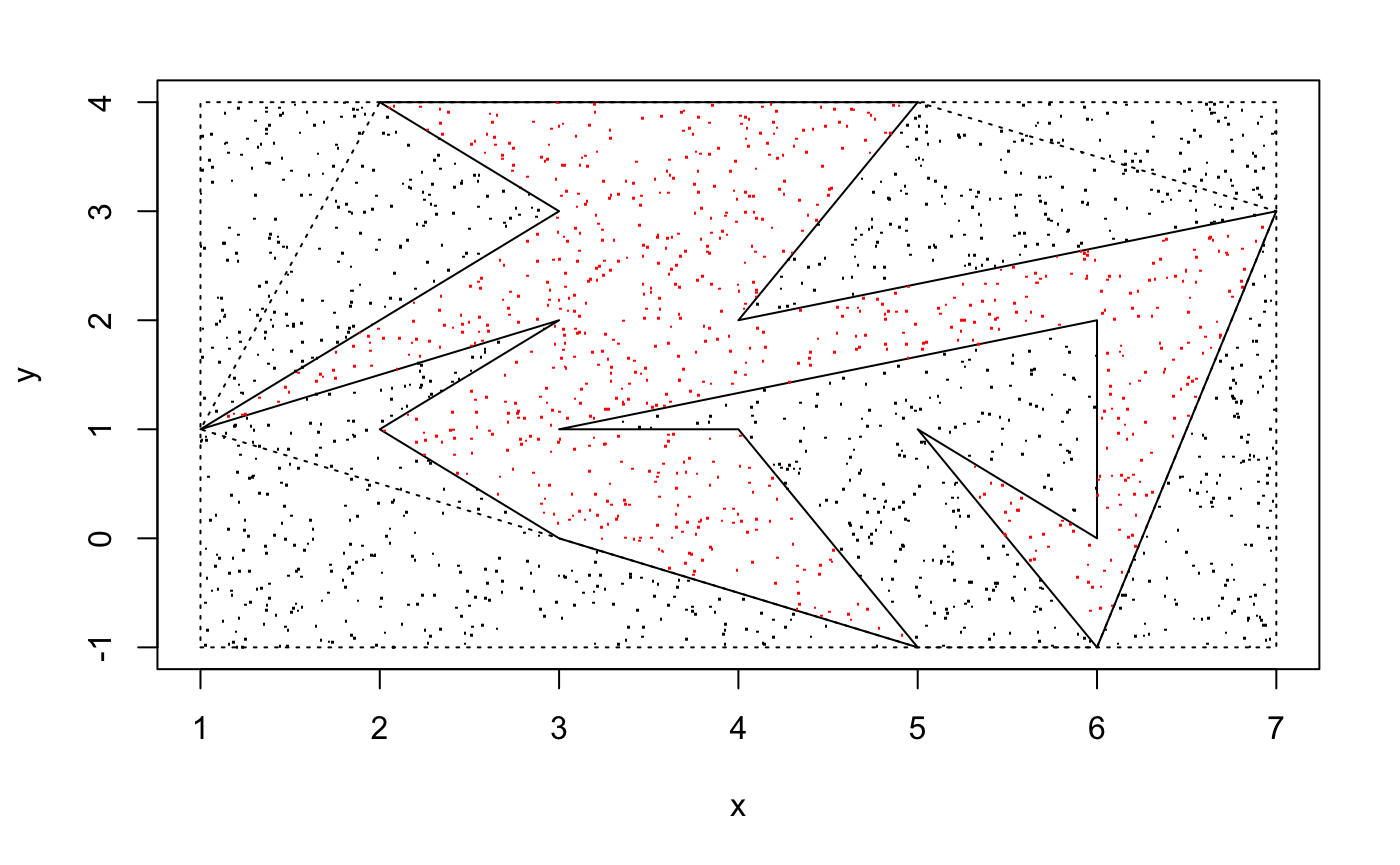
## [1] 11.91Compare two figures above, we can see the second function successfully get rid of all the points that's inside the polygon in-between that is concave. Even if the polygon is very complex, the error will be reduced and hence we can get more accurate answer.
Remember, this function is not very efficiency, as the point in polygon algorithm above is laggy. In Part 2, we will refer some popular algorithms and rewrite the point in polygon function, to make it possible to detect a point inside whether convex, concave or self-intersecting polygon.
© Group 18